Understanding Optimisers Through Hessians

Introduction

During my recent autodiff library project I got the opportunity to implement common optimizers from scratch. Furthermore, while investigating the vanishing gradient problem I benefited greatly from diving deeper into concepts that I had previously accepted based on intuitive arguments alone. To further this pursuit of a deeper understanding of deep learning fundamentals, I decided to question my grasp of optimisers.

In the past, I have had momentum explained to me as a way to “have the optimisation more accurately simulate a ball rolling down a hill.” Indeed, adding momentum does make the dynamics analogous to applying (semi-implicit) Euler’s method to a ball rolling down a hill. However, this begs the question: why should this be strived for? What makes the physics of a rolling ball inherently superior for optimisation?

Similarly, I have always had Adam explained to me as a way to “give additional priority to infrequent coordinate updates.” I have never found this motivation very convincing, this sounds like a recipe for instability and overfitting when there are anomalous data points in the training data. I can think of just as many cases where this approach would have a deleterious effect on convergence.

Surely, there is something deeper going on that better explains the general efficacy of both of these approaches.

Deriving Gradient Descent

Suppose we have some loss function and our current parameter vector is . Now suppose we want to take some step in parameter space to maximise our reduction in loss. First, Lets assume our loss function is continuous in its first derivative, then Taylor’s theorem states that we can expand our function about our current parameter value relative to some perturbation as follows:

Which means that for small step sizes, i.e. such that is small, we can make the first order approximation that:

Which means that if we want to maximise the reduction in loss, then we want to minimise the quantity:

The above is the inner product between our perturbation and the gradient. It follows from the Cauchy-Schwarz inequality that minimisation of the above quantity is achieved by pointing our perturbation in the opposite direction of the gradient. Therefore, in order to achieve our desired minimisation, while ensuring our first order approximation valid, we set our perturbation to:

This is the basis for gradient descent, which can be seen as an iterative loss function reduction procedure, which is defined as follows:

Convergence of Gradient Descent

Suppose our current parameter value is close to a local minimum . Then we can consider our parameter vector to be some perturbation about the local minimum, i.e . Assuming second order continuity of our loss function, we can now use a Taylor expansion about our local minimum as follows:

We now note that since we are expanding about a local minimum, it follows that . Furthermore, we will assume that we are sufficiently close to the local minimum such that higher order effects can be ignored, i.e. . Therefore, we have

which gives a second order approximation for the gradient of

Since the hessian is symmetric and real valued, it follows from the spectral theorem that there exists some orthonormal basis which are eigenvectors of . Furthermore, the orthonormal eigen vector’s eigenvalues are non-negative by virtue of the fact that is a local minimum. Therefore, we can expand our perturbation in terms of this orthonormal basis as follows:

Where is the component of along . If we now apply our second order approximation for the gradient to the above expansion we see that

We can now revisit our expression for gradient descent with the above expansions in mind.

Which can be understood as a shrinkage of the eigen-components of our perturbation by a factor of each iteration. When expanding this to the the base case of our initial perturbation, this gives the equation:

Therefore, it follows that so long as we choose a such that:

Then we will get linear convergence of our perturbation to the zero vector, which is equivalent to linear convergence of our parameter to the local minimum. Importantly, each of the eigen-componenents converge to zero independently, and at different rates for a given . Furthermore, we are okay with oscillation, i.e. , so long as the magnitude of the perturbation is decreasing after each iteration.

Additionally, we notice that is monotonically decreasing in terms of , i.e.

Importantly, for nonzero , we have

Immediately, this tells us we achieve convergence if and only if . Which places a maximum value of equal to

The Steep Valley Problem (ill-conditioning)

Our previous equations present a rather glaring problem, if the eigenvalues of our hessian are separated by orders of magnitude, then a valid choice of such that we can achieve convergence can lead to drastically different rates of convergence for the components

Therefore, given that convergence requires all eigen-componenets to converge, it follows that the rate of convergence for our whole procedure is given by

To find the optimal value of lets consider how this expression changes as we vary . For small both quantities are positive, so we start with . As we increase there is some point at which hits zero, further increases of will cause to increase (not decrease). We now have a situation where has a positive and larger magnitude gradient than . Therefore, at some point between , the two rates will intersect, i.e. . This intersection point will represent the minimum value for , since prior to this point was the rate setter, meaning that was monotonically decreasing for . Meanwhile, after this intersection point will be the rate setter, meaning that will monotonically increase for . Importantly, this means that it is not only permissible for the maximum eigenvalue component to oscilate, it is desirable for optimal convergence.

To find this intersection point we observe that it will occur for and , meaning that we are solving for in the following equation:

The associated value of will be equal to:

Where we have identified the conditioning number of our hessian , which is equal to the ratio of our largest eigenvalue to our lowest eigenvalue.

As a concrete example, consider and . Looking at a plot of , and against , we see that and are indeed the optimal values for and the associated overall rate of convergence.

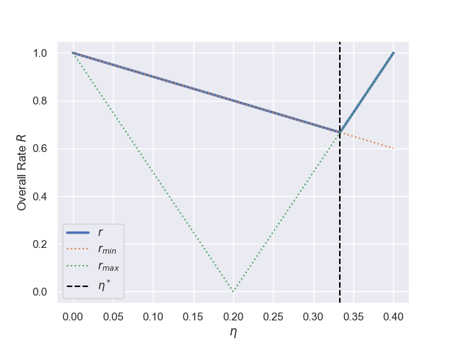
We notice that if we have a very large conditioning number, the associated overall rate of convergence will be very slow, i.e. . In fact, this could be so prohibatively slow as to completely stall convergence for practical purposes, under such circumstances we would say the optimisation problem is ill-conditioned. Although, such a scenario is more commonly referred to within the deep learning community as a steep valley problem, where the loss landscape is being compared to a valley with step sides (large ) relative to a shallow gradient (small )orthogonal to the valley slopes.

Momentum

With the context of the ill-conditioning problem setup, we are now ready to discuss momentum. Momentum modifies our iterative process by having our gradients directly update a momentum term, rather than the parameters directly. In this sense the gradients now act much more like an acceleration, i.e. something that changes velocity, rather than an instantaneous velocity. Furthermore, we introduce a hyper-parameter which puts limits on how much the gradients can accumulate. The exact form of the update rule with momentum is given below:

A common variant of momentum is Nesterov momentum, this changes the way in which the momentum is calculated as follows:

The key difference is that we evaluate the gradient where the momentum will take us. This makes sense if the size of the momentum term is much larger than the gradient itself. In such circumstances the naive approach leads to gradient evaluations that are irrelevant relative to where the parameter will end up after the update. It makes much more sense for the gradient to act as a small correction term which is applied after momentum moves the parameter.

Lets now study some consequences of the above modification, relative to our ill-conditioned optimisation problem. First lets consider our small eigenvalue component. Given that this component is being updated on an axis of low curvature relative to the update length-scale set by the large eigenvalue component, it follows that the updates at each step are roughly constant, i.e.

We can now use this in combination with our definition of momentum to see that

Which means that a value corresponds to allowing the gradient updates for the slow components to amplify by a factor of 10. However, setting too high should be cautioned against, else we could have a scenario where the minimum eigenvalue axis builds up so much momentum that it overshoots the local minimum and enters a new basin, which will likely face a similar issue, i.e. our optimiser will struggle to converge. A well set effectively acts as a way to artificially increase and therefore alleviate the ill-conditioning problem.

From a physics perspective we could compare to a drag/friction term, in which case the above calculation would be analogous to a terminal velocity calculation.

We can now apply a similar sort of analysis to our maximum eigenvalue component. We notice that for an ill-conditioned problem we have . Therefore, as an approximation for the effects of momentum on the maximum eigenvalue component case, we will consider the limiting case of pure oscillation. In this case we have

Therefore, momentum has a small damping effect on oscillations. Reading too deeply into the above result should be cautioned against, since the fact that oscillations are being damped invalidates the assumption that we can approximate the gradient as an oscillating constant, i.e. the gradient will change as we go down the steep valley. Again, this acts to artificially reduce and aid the ill-conditioning problem

Adaptive Learning Rate

Motivation

Our previous analyses have been predicated on the assumption that we have set , such that we are able to achieve convergence. Such a task is trivial when we know the hessian evaluated at the local minimum. However, for practical tasks we don’t even know the local minimum, let alone its hessian. Therefore, before we even start training our model, by selecting some value of as a hyper-parameter, we are essentially selecting some subset of minima that the model can converge to. This might not be problematic in itself, in fact we could view a preference against steep minima as an inductive bias of our optimisation procedure/model.

Nonetheless, lets say we did want to increase the set of minima that we are capable of converging to. Ideally we want to do this without decreasing , which could lead to prohibitively slow convergence. Our previous analysis showed that the ability of our optimiser to converge was governed by the largest eigenvalue components of a local minimum’s hessian, i.e. we could achieve convergence so long as growing oscillations were prevented. Recall, that the step size along a given eigenvector while performing gradient descent is equal to

Ideally, we would be able to come up with some procedure for estimating , such that we could divide our gradient updates by this estimate and have our linear convergence rate equal for all our eigen-components. However, even if we knew the eigenvectors of the hessian, there is no way to disentangle from based solely on observations of . A next best option would be to attempt to estimate some scale . In which case, we could divide our naive update by this estimate and achieve a gradient update:

This does not achieve the same linear convergence guarantees as before, and would lead to “oscillation” about the true local minimum, i.e. not truly converge to the local minimum. However, assuming our estimation procedure was effective, it would let us get within a radius of an arbitrary local minimum. Importantly, for adaptive methods is much more akin to a direct step size rather than a scaling factor for the gradient. For this reason, smaller values of are typically recommended for methods using adaptive learning rates compared to standard gradient descent.

AdaGrad

One of the first approaches to attempt to tackle the above was Adaptive Gradients (AdaGrad). It simply estimated the scale parameter using the square root of the cumulative sum of gradients squared. Additionally, since we do not know the local minimum’s eigenvectors, we cannot scale across these specific directions. Instead, we simply scale across the coordinates of whatever arbitrary coordinate system our parameters are defined in, which has empirically been shown to work well. The full update rule is as follows:

This was a good first approach, but it does not adapt well to the scenario of our local minimum changing, potentially due to overshooting, since now a previously large component might be very small and need special attention. Furthermore, although the cumulative scale overcomes the “oscillation issue” demonstrated in the motivation for this section, it is too aggresive and leads to training hatling.

RMSProp

Root Mean Square Propagation (RMSProp) builds on AdaGrad by looking at an exponentially weighted estimate of the root mean square gradients. This fixes the issue regarding training halting. The full update rule is given below:

Adam

Adam (Adaptive moments) was introduced in the paper “Adam: A Method for Stochastic Optimization”. Indeed, its motivation was to stabilise training for stochastic error functions, e.g. those resulting from mini-batch gradient descent and dropout regularisation. The focus of the paper was on robust estimation of the first and second order moments of the gradients using exponentially weighted averages. This is performed as follows:

Furthermore, a de-biasing step is applied, which is used to de-bias these first and second order moment estimates of the gradients relative to their zero value initialisation.

Notice, that this effect becomes negligible as .

Finally, the update rule is given by the following:

A common misconception is that Adam is “RMSProp plus momentum”, this being in spite of the paper stressing that this algorithm is distinct from RMSProp plus momentum, which is a perfectly valid optimiser that can be used within most deep learning frameworks. Importantly the “momentum” term in Adam does not perform accumulation, to see this notice that the “momentum” term for some constant gradient update would equal:

In other words, it would not accumulate. Indeed, the purpose of the “momentum” term is not accumulating consistent gradient updates. Instead, as stated above, the motivation for the Adam paper was to provide a more stable training experience for stochastic error functions. Therefore the role of the “momentum” term in Adam is that of gradient smoothing over a potentially noisy training procedure.

A further nice property of Adam is that it allows us to use Jensen’s inequality to further our analysis. Recall that if is a convex function then it follows that:

Importantly, this means that

Which means that if our first and second moments are estimated correctly, then our gradient step size is bound from above by , which is exactly the behaviour that adaptive learning rate methods strive for. Furthermore, it is common to set and , i.e. have the second order moment have a longer memory than the first order moment. This has the effect of gradually reducing the effective learning rate as the parameter approaches the local minimum, since our second order moment is being estimated with previous regions of the loss landscape that had higher gradients. In practice this means that Adam enjoys favourable convergence speed and is able to overcome the “oscillation issue”.

Experiments

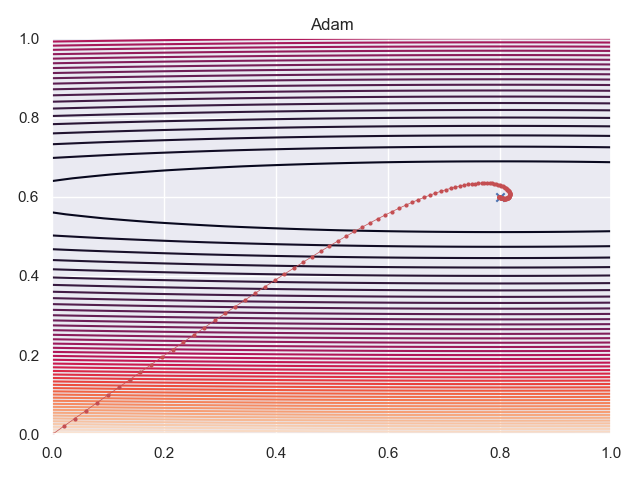
To finish this investigation off I decided to run some experiments. I looked at a 2 dimensional quadratic optimisation problem. The associated elliptic paraboloid was centered at and had a diagonal hessian in the parameter coordinate system with eigenvalues and , i.e. . A number of different optimisers were evaluated on their ability to update a parameter, whose initial position was set to the origin, within a radius of the global minimum.

MINIMA = torch.Tensor([0.8, 0.6])

LAMBDA_MIN = 1
LAMBDA_MAX = 100

ETA_OPT = 2 / (LAMBDA_MIN + LAMBDA_MAX)
ETA_MAX = 2 / (LAMBDA_MAX)


def f(p):
    H = torch.Tensor([[LAMBDA_MIN, 0], [0, LAMBDA_MAX]])
    delta = p - minima

    return delta @ H @ delta / 2

def optimiser_experiment(
    experiment_name: str,
    optimiser: Callable[..., torch.optim.Optimizer],
    *args,
    **kwargs,
):
    p = torch.tensor([0.0, 0.0], requires_grad=True)

    opt = optimiser([p], *args, **kwargs)

    p_history = [p.detach().clone()]
    f_eval = 1
    epoch = 0
    while f_eval > 1e-6 and epoch < int(1e4) and abs(p[0]) < 5 and abs(p[1]) < 5:
        f_eval = f(p)
        f_eval.backward()
        opt.step()
        opt.zero_grad()
        p_history.append(p.detach().clone())
        epoch += 1
    p_history = torch.stack(p_history, axis=0).detach()

    if not torch.isnan(f_eval):
        print(f"{experiment_name} - {epoch}")
    else:
        raise RuntimeError("Function evaluation overflowed.")

    xs = torch.linspace(min(min(p_history[:, 0]), 0), max(max(p_history[:, 0]), 1), 100)
    ys = torch.linspace(min(min(p_history[:, 1]), 0), max(max(p_history[:, 1]), 1), 100)
    zs = [[f(torch.Tensor([x, y])) for x in xs] for y in ys]

    plt.figure()
    plt.title(experiment_name)
    plt.contour(xs, ys, zs, levels=50)
    plt.scatter(minima[0], minima[1], marker="x")
    plt.plot(
        p_history[:, 0],
        p_history[:, 1],
        "r-",
        linewidth=0.5,
        marker=".",
        markersize=4,
    )
    plt.savefig(f"results/optimisers/{experiment_name}.png")

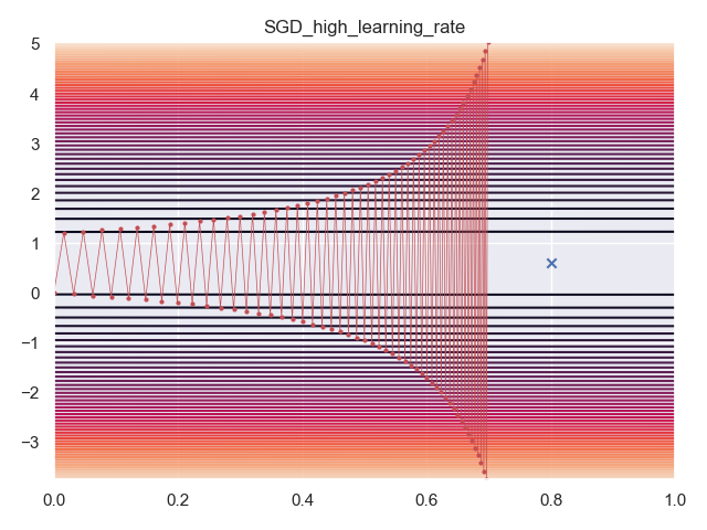
SGD - Learning Rate Too High

First, I used SGD with a learning rate of , this led to training that diverged.

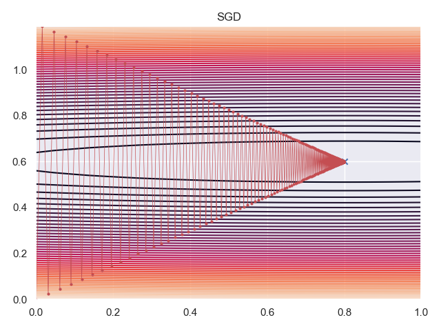
SGD

Next, I used SGD with a learning rate of , this converged after 420 iterations.

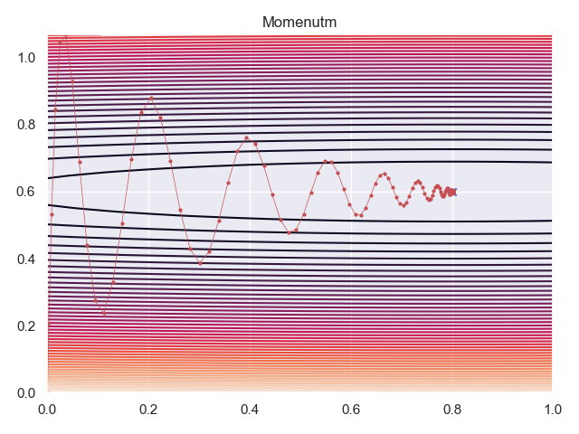
Momentum

SGD with and , was able to converge in 137 epochs.

Adam

Adam with a learning rate of , and was able to converge in 117 epcohs.

Recommendations

Adam with the defaults of and is a good default optimiser to use. However, it is possible that avoiding steep minima is a favourable inductive bias for your model/optimiser to have, and as such it is possible that a simple SGD with momentum optimiser ends up being optimal for your given problem.

References

1. Bishop CM, Bishop H. Deep learning: Foundations and concepts. Springer Nature; 2023 Nov 1.
2. Géron A. Hands-on machine learning with Scikit-Learn, Keras, and TensorFlow: Concepts, tools, and techniques to build intelligent systems. ” O’Reilly Media, Inc.”; 2022 Oct 4.
3. Kingma DP, Ba J. Adam: A method for stochastic optimization. arXiv preprint arXiv:1412.6980. 2014 Dec 22.