Backpropagation A Modern Explanation

Introduction

Manual differentiation is prone to errors and does not scale to functions that involve thousands of parameters, e.g. neural networks. This necessitates procedures which are able to take functions and generate evaluations of their gradients.

Automatic differentiation (autodiff) describes efficient algorithms for calculating the gradients of supplied functions using nothing more than their implementation, i.e. their forward pass information. Furthermore, modern autodiff frameworks are often able to handle dynamically defined functions, whose behaviour changes during runtime, i.e. they can handle dynamic looping and branching logic.

More specifically autodiff implementations operate on the compute graph of some supplied function. Although this “compute graph” subtlety is often abstracted away in modern frameworks, a user simply needs to define a high level function and the associated compute graph will be built in the background. The key improvements, in terms of efficiency, lie in the intelligent ways in which autodiff frameworks utilise previous computations in the compute graph.

Backpropagation

We can think of backpropagation as a specific example of automatic differentiation. In this article we will refer to backpropagation as the application of reverse mode automatic differentiation to scalar valued loss functions, whose value depends on the inputs (parameters) of a neural network. I believe this definition encapsulates the core of what most modern deep learning frameworks mean when they refer to backpropagation.

The Problem With Typical Introductions to Backpropagation

Most deep learning practitioners are first exposed to automatic differentiation when they study the backpropagation algorithm for optimising layered neural networks. For context, we start with some feed-forward neural network which can be split into a sequence of layers.

For ease of derivation, these layers are usually constrained to take on the following structure:

Where we call the activation function for the layer. Under these constraints, the above function composition can be rephrased in terms of an iterative procedure in terms of transforming the output vectors from one layer to the next layer.

Where we call the post-activation and the pre-activation of layer . The input to the network is and the output is

After defining the above setup, most machine learning texts then go on to derive the backpropagation algorithm. Unfortunately, it is hard to come by a consistent definition of “backpropagation”, some texts describe it as the algorithm for getting derivatives for networks like the one defined above, while others define it as the full optimisation procedure for neural networks (including gradient descent). Nonetheless, at the intersection of these treatments of backpropagation, are the following iterative equations for calculating derivatives:

Unfortunately, this is where most introductory texts end their discussion on automatic differentiation. I believe this does a huge disservice to budding deep learning practitioners. It leaves them thinking that in order to perform gradient descent on their networks, they must define them in a way amenable to the above procedure, i.e. constraining their network architectures to sequential layers that conform to the above layer function forms. Suddenly, every new neural network compute unit they learn about needs to fit into the above layered framework. For example, convolutional layers are thought of in terms of sparse matrix multiplications with weight sharing, concatenation layers are framed in terms of combining previously block diagonal matrix computations, batch normalisation layers correspond to various multiplications by diagonal matrices, etc. These misconceptions might be admissible if they remained in the realm of the abstract, but many of these misconceptions, if taken to concrete implementations, would lead to very inefficient procedures.

I believe the reliance on this example is a hangover from an era where such architectures did encapsulate the vast majority of networks under study. Additionally, its emphasise on a sleek formula that could, in theory, be hand calculated is also reminiscent from a time when compute was less available. Furthermore, I would argue that the above formulation is antithetical to the objectives of automatic differentiation. The main objective of automatic differentiation is to move away from a world where we have to manually derive derivatives. Armed with the toolkit of automatic differentiation, the problem solving process for getting the derivative of a fully defined forward implementation, should not be to try and get some cleverly crafted set of iterative equations, it should be to pass the forward implementation to the automatic differentiation engine… That is not to say that the above formulation is not useful, for example, it provides useful insights into the vanishing/exploding gradients problem. I am simply advocating for a much greater emphasis to be placed on the algorithmic automations provided by automatic differentiation.

Background

Before discussing Automatic Differentiation further, it is worth discussing simpler alternatives first. This will help us introduce some key concepts and gain a greater appreciation for how automatic differentiation builds on these approaches. Throughout these discussions we will be tackling the problem of finding the derivatives of functions with respect to their inputs. It should be stressed that neural networks are deterministic functions, whose inputs are their input vector and their parameters, the latter type of input is often obscured by common notation.

Numerical Differentiation

We recall from the definition of the derivative that:

This means we can approximate partial derivatives by adding a small amount to their evaluation and subtracting the original evaluation, and then dividing by the shifted amount.

It can actually be shown that a better approximation is achieved by taking symmetric differences as follows:

Unfortunately, the above procedure is quite limited by the precision of floating point numbers. Furthermore, if we have inputs, then the above procedure will require computations, one for each input being perturbed while the others remain constant. For a neural network where the inputs are the parameters of the model, then the compute of an individual forwards pass also scales , this resulting in a procedure to get all the gradients. Which is prohibitively slow for large networks.

Nonetheless, numerical differentiation is a quick and easy approach that can be a serve as a useful reference implementation that you can test your more complex implementations against.

Symbolic Differentiation

Symbolic differentiation is a useful stepping stone for us to understand automatic differentiation, since it introduces the concept of a compute graph .

We can think of a compute graph as the result of a recursive procedure on our function, whereby we break it down into the more foundational functions from which it is composed. The result is a set of vertices representing intermediate values and a set of edges representing composition. More specifically, internal vertices are associated with the outputs of simple functions, while external vertices (leafs) represent either inputs or constants, i.e. compute units which cannot be broken down further.

For example, the compute graph for the following function:

Is given by:

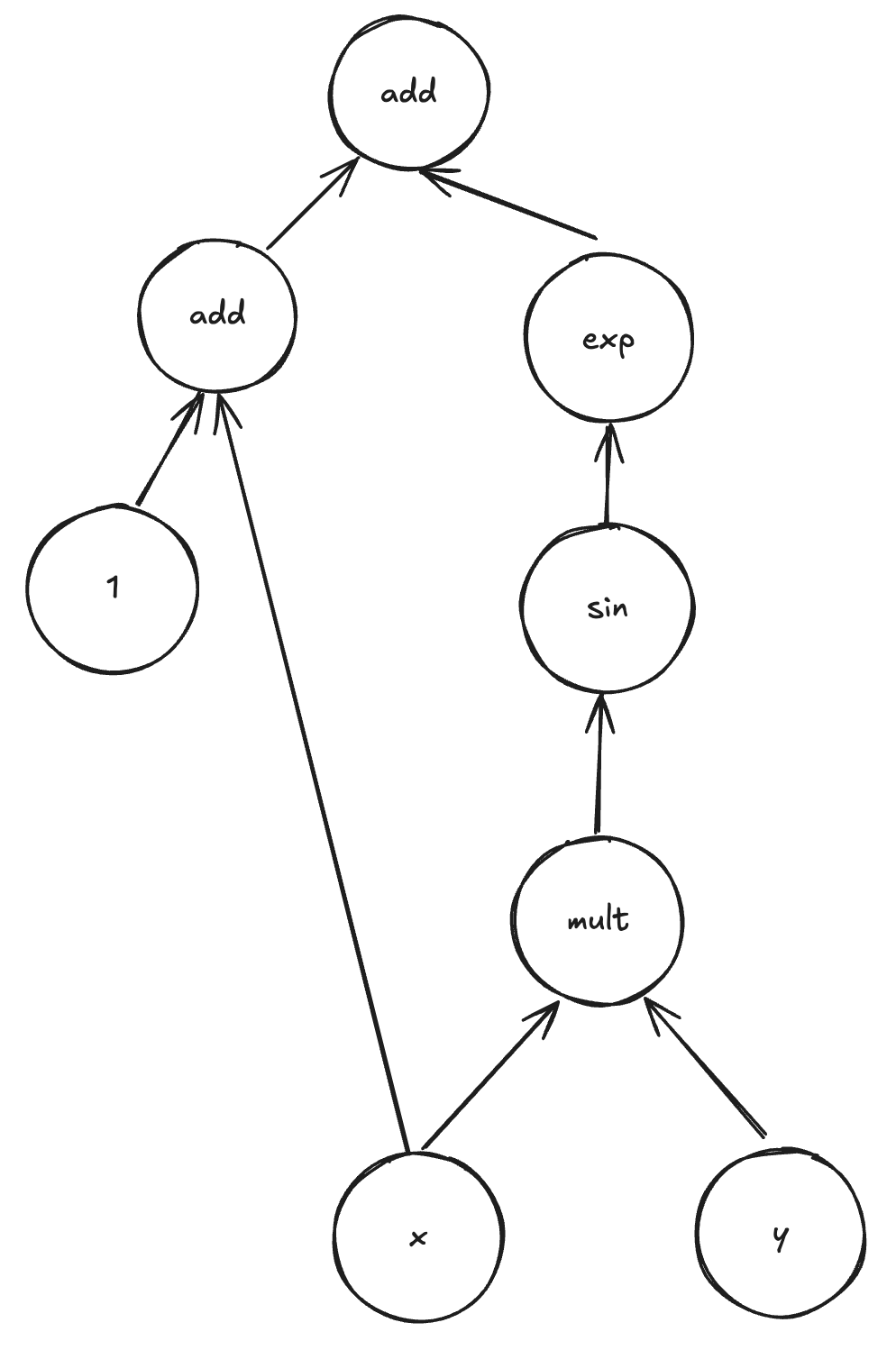
We can manually derive the derivatives by using the rules of calculus:

However, if we actually break down our process of manually solving this derivative, then we will realise we were performing something very similar to traversing our original compute graph, i.e. we go through our original expression recursing through the layers of composition. If we have a simple arithmetic expression then we distribute the derivative using linearity, if we are faced with product we use the product rule, if we are faced with more complicated composition we use the chain rule… Symbolic differentiation simply systematises the above procedure by traversing the compute graph and producing a new compute graph for the derivative.

For example, the rules of symbolic differentiation applied to the original compute graph would result in the compute graph listed below. Here we have use to denote the derivative of symbol with respect to some variable. For example if we wanted to use this compute graph to find then , and .

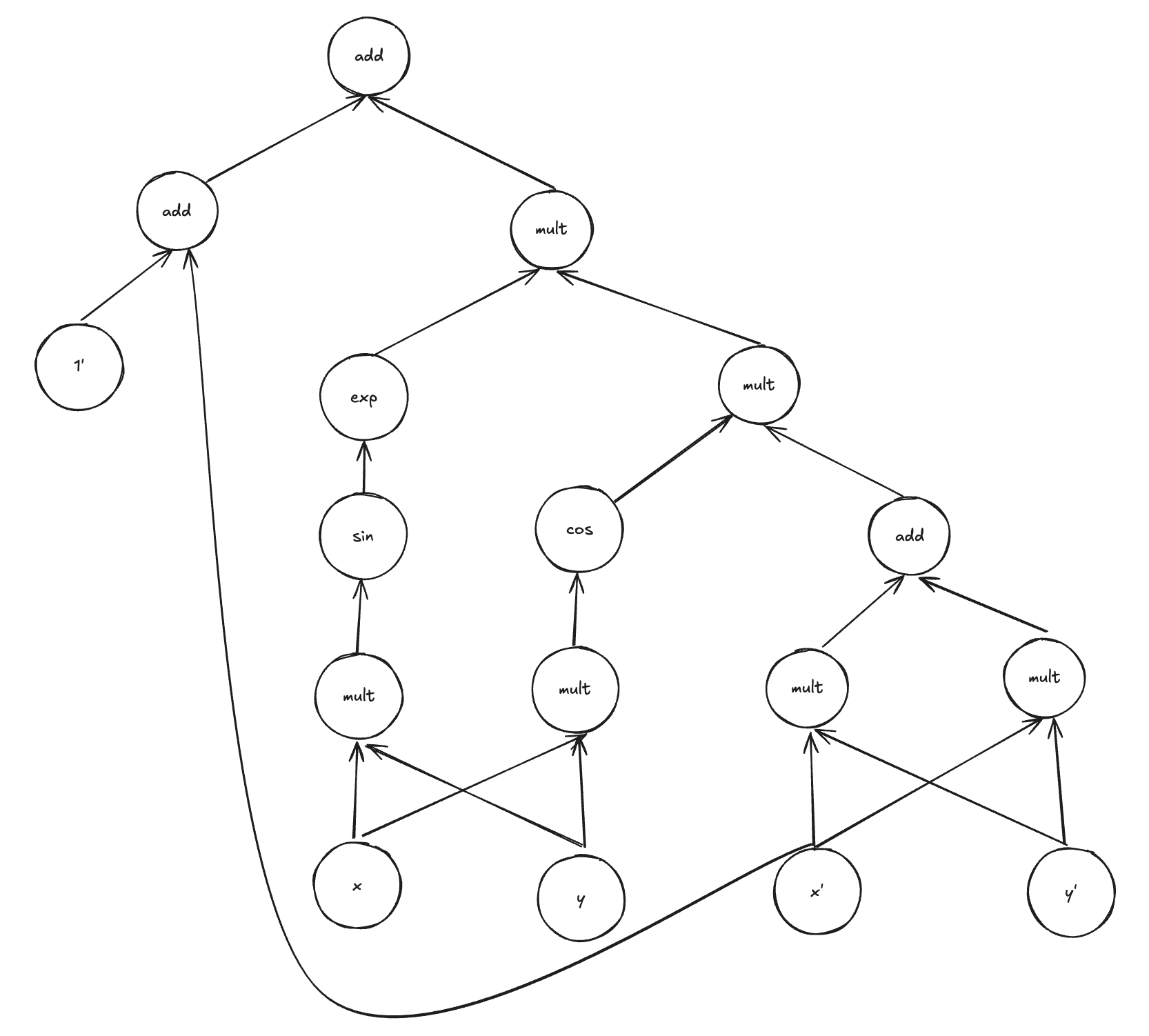
The main disadvantage of this approach is that the complexity of the derivative compute graph is often much higher than the original compute graph, which stems from the branching caused by applications of the chain and product rule. Furthermore, this procedure does not efficiently reuse previous compute.

These inefficiencies are not important relative to symbolic differentiation’s key objective, which is to produce a human readable output for the derivative in terms of the symbols in the originally supplied expression (this is the technology behind mathematica). This human readable part is usually implemented by an additional pass through the produced graph where symbols are collected. Furthermore, this requirement that it needs to be passed a mathematical expression makes them ill suited for computer programs with dynamic runtime behaviour, such as dynamic branching and looping.

Automatic Differentiation

We can view automatic differentiation as a refinement on symbolic differentiation, taking into account our requirement for efficient computation rather than human readable output. Furthermore, it is usually implemented to allow dynamic construction of the compute graph during runtime.

Forward Mode

In forward mode we augment all values in our compute graph with values which represent the vertex’s gradient with respect to some fixed input/vertex. In other words each vertex in our compute graph now stores two values , called the primal value and the tangent value of a vertex. More specifically, for a given forward mode computation we define the tangent values of our vertices relative to some input

The objective of forward mode autodiff is to devise a procedure to pass gradient information forward with the primal values during the forward pass. The key to doing this is to notice that , i.e. is completely specified by the values of its parents in the forward mode compute graph. We can use this alongside the chain rule to find the total derivative of as follows

Importantly, this says that we can get the tangent values of children using the tangent values of parents. Which means we have replicated the desired flow of information and can perform this step alongside standard forward propagation. We now need to simply repeat this procedure until we get to the end of the network, at which point we will have found the derivative of the output with respect to the input in question.

In order to find the gradient of a given parameter we simply one hot encode its tangent and pass this through the network, i.e. to find the gradient of we pass , since this is what the tangent values are equal to when we are performing differentiation with respect to .

Importantly, we have devised a method which allows us to compute derivatives using a procedure with comparable computational complexity to the forward pass, i.e. we have removed the issue associated with symbolic differentiation where the compute graph for the derivative explodes. However, the main issue with forward mode automatic differentiation is that a single pass only gives us the derivative for one input. This means that it has a similar problem to numerical differentiation where it requires forward passes, each with compute requirement, leading to a procedure for getting all the gradients. The main improvement relative to numerical differentiation is that it has better numerical stability.

Reverse-mode automatic Differentiation (Backpropagation)

Forward propagation set off with the objective of finding arbitrary vertex derivatives with respect to a specific vertex, i.e.

we then specialised this to the desired case of being the output vertex.

However, our actual objective is to get the gradients of a specific vertex (output) with respect to arbitrary vertices (inputs). To this end, we now define the “adjoint” vertex values:

which are similar to the tangent values, but now the vertex being differentiated is fixed, while the differentiating vertex varies. We now seek to find some method for calculating for the entire graph using known pairs of these values in the graph.

The trick to solving this problem is to notice that if we are given the children of some vertex , then it follows that we can reparameterise the output in terms of these children and remove explicit dependence, i.e.

This empowers us to use the total derivative and chain rule on our adjoint variables

Which shows that we can use the adjoint values of child vertices to calculate the adjoint values of a parent vertex.

Importantly this allows us to compute all the gradients in as opposed to , this is because the end result of reverse mode automatic differentiation will be evaluations of for each vertex. To get the derivative of with respect to a given input/vertex simply look at the value of .

The only downside is that we need to store all the the intermediate computations of the forward pass, i.e. we incur space complexity. This is so that the vertex-wise gradients can be evaluated on the backwards pass, i.e. we need ‘s values in order to evaluate . However, this penalty in space complexity is usually well worth the reduction in time complexity for large neural networks.

Automatic?

In the introduction we promised a procedure that could automatically compute derivatives of functions given nothing more than the forward pass of a function. Indeed, given the starting values for inputs () and for the outputs () we can use the forward and backward mode autodiff equations to propagate these values throughout the compute graph.

However, this begs the question, how do we “automatically” get the edge weights, corresponding to the derivatives of children with respect to parents, i.e.

It appears that we need to manually specify these alongside our forward propagation, i.e. we lied in our original assertion. However, if you have ever used an autodiff framework (e.g. PyTorch, TensorFlow or JAX) then it is likely you have not had to manually pass in such derivatives.

This is because under the hood all of the “functions” defined within these frameworks are actually objects, whose default call corresponds to a “forwards” implementation. However, tacked onto all these functions is a reverse mode that the maintainers of the framework have implemented for all of the most popular functions (e.g. arithmetic, trigonometric functions, exponential, …).

These pre-implemented functions will cover you in the vast majority of cases. However, in the rare circumstance that the maintainers have not implemented some function that you need, then most frameworks will provide an interface which you can implement such that you can define user defined functions which work within their framework. The only caveat being that you will have to manually implement the derivative of these user defined functions.

For a full walkthrough on how to build a library that implements the above functionality, see my blog post.

Revisiting the Layered Network

We started this article with a criticism of the typical way in which backpropagation is introduced, whereby the focus is on the specific application to a layered neural network. In this article we took an alternative approach, we focused on the general framework of automatic differentiation, not a specific application.

We will now come full circle and apply this general framework that we have developed to the specific example of a layered neural network. Recall, our layered neural network obeys the forward equations:

We now turn our attention to the adjoint variables , which are equivalent to vertex sensitivities in our original treatment . The reason we look into these quantities instead of the more direct is because ultimately we are looking for an iterative expression we can apply to the compute graph, and the former adjoint variables are leafs, i.e. dead ends. Our backwards autodiff equation now tells us that

Or in vector form

Now all that remains is to go one connection down into the compute graph and get the derivatives with respect to the parameters that feed into the pre-activations:

Which is equivalent to the result shown in our original discussion on backpropagation.

References

1. Bishop CM, Bishop H. Deep learning: Foundations and concepts. Springer Nature; 2023 Nov 1.
2. Géron A. Hands-on machine learning with Scikit-Learn, Keras, and TensorFlow: Concepts, tools, and techniques to build intelligent systems. ” O’Reilly Media, Inc.”; 2022 Oct 4.