Hardware Accelerated Bootrapping

Introduction

Following my investigation into bootstrap confidence intervals, I set out to run some simulation experiments to observe how the coverage of these confidence intervals approached their nominal levels. I noticed that there didn’t appear to exist a popular JAX implementation for this functionality, so I took it upon myself to implement these methods inside a package I am calling statax. I think JAX is uniquely well suited for bootstrapping due to its ease of vectorisation via vmap and its jit capabilities, which are especially useful for repeated computation of a supplied statistic function.

While, it is true that the scipy.bootstrap function will allow you to enable vectorisation, this functionality is not as easily utilised since the burden is on you to pass scipy.bootstrap an efficiently vectorised implementation of your statistic. Nonetheless, even in the scenario where we pass scipy.bootstrap a vectorised statistic there is still utility in using a JAX implementation. This is is shown below where JAX allows us to easily vectorise a coverage experiment built on top of the bootstrap procedure, and as such achieve a >4x speedup relative to the same experiment using scipy.bootstrap. Obviously, this speed up is even more drastic when we are not able to pass scipy.bootstrap an easily pre-vectorised statistic.

N_SIM = 1000
N_SAMPLES = 100
N_RESAMPLES = 2_000


def scipy_bootstrap(seed: int = 42):
    rng = np.random.default_rng(seed)
    data = rng.normal(size=N_SAMPLES)

    res = bootstrap(
      (data,), 
      np.median, 
      confidence_level=0.95, 
      n_resamples=N_RESAMPLES, 
      vectorized=True, 
      method="BCa",
    )

    low, high = res.confidence_interval
    contains = low <= 0 and high >= 0

    return contains


def simulate_scipy():
    res = 0
    for i in range(N_SIM):
        res += scipy_bootstrap(i)
    return res / N_SIM


@jit
@vmap
def statax_bootstrap(key: jax.Array):
    data = random.normal(key, shape=(N_SAMPLES,))

    bootstrapper = BCaBootstrapper(jnp.median)
    bootstrapper.resample(data, n_resamples=N_RESAMPLES)

    ci = bootstrapper.ci(confidence_level=0.95)
    contains = jnp.logical_and(ci[0] <= 0, ci[1] >= 0)

    return contains


def simulate_statax():
    key = random.key(0)
    res = jnp.sum(statax_bootstrap(random.split(key, N_SIM)))
    return res / N_SIM


if __name__ == "__main__":
    logging.basicConfig(level=logging.INFO)

    scipy_time = timeit(simulate_scipy, number=100)
    logging.info(f"scipy time: {scipy_time:.2f}")

    statax_time = timeit(simulate_statax, number=100)
    logging.info(f"statax time: {statax_time:.2f}")

    logging.info(f"{scipy_time / statax_time:.2f} factor speedup.")

INFO:root:scipy time: 316.69
INFO:root:statax time: 77.94
INFO:root:4.06 factor speedup.

Coverage Experiment

To test the coverage of different bootstrap confidence interval methods, I simulated n_sim bootstrap confidence interval generations for each bootstrap confidence interval generation procedure. I then calculated what percentage of the time these confidence intervals contained the true statistic. This ratio was then used as an estimate for the coverage of that confidence interval generation procedure for a given $n$.

class SamplingDistribution(Protocol):
    def __call__(self, key: jax.Array, n: int) -> jax.Array: ...


class StatisticFn(Protocol):
    def __call__(self, data: jax.Array) -> jax.Array: ...

def estimate_coverage(
    bootstrapper_constructor: Callable[..., Bootstrapper],
    sampling_distribution: SamplingDistribution,
    statistic_fn: StatisticFn,
    confidence_level: float = 0.95,
    n_sim: int = 10_000,
    n_samples: int = 100,
    n_boot: int = 2_000,
    batch_size: int = 1000,
    seed: int = 0,
):
    key = random.key(seed)

    key, subkey = random.split(key)
    true_statistic_value = statistic_fn(sampling_distribution(subkey, 1_000_000))

    bootstrapper = bootstrapper_constructor(statistic_fn)

    @jax.vmap
    @jax.jit
    def confidence_interval_simulation(key: jax.Array) -> tuple[jax.Array, jax.Array]:
        key, subkey = random.split(key)
        data = sampling_distribution(subkey, n_samples)

        key, subkey = random.split(key)
        bootstrapper.resample(data=data, n_resamples=n_boot, key=subkey)

        ci_low, ci_high = bootstrapper.ci(confidence_level=confidence_level)
        return (true_statistic_value >= ci_low) & (true_statistic_value <= ci_high), ci_high - ci_low

    covered_count = 0
    total_length = 0
    i = 0
    while i < n_sim:
        logging.debug(f"Batch: i / {n_sim}")

        current_batch_size = min(batch_size, n_sim - i)
        key, subkey = random.split(key)

        is_covered, length = confidence_interval_simulation(random.split(subkey, current_batch_size))
        covered_count += jnp.sum(is_covered)
        total_length += jnp.sum(length)

        i += batch_size
    coverage = covered_count / n_sim
    average_length = total_length / n_sim

    return coverage, average_length

Simple Statistic

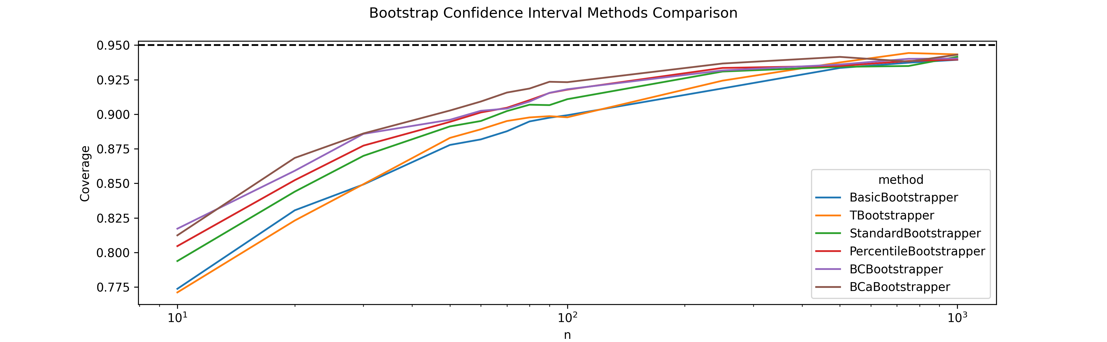
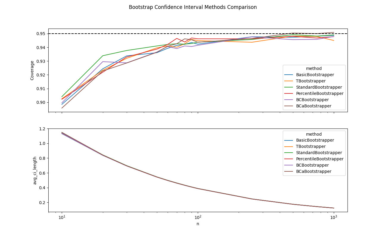
As an end-to-end test for my different bootstrap confidence interval estimation procedures, my first experiment was on estimating the median of a normal distribution. As can be seen below, all methods start with a true coverage of $\approx 90\%$ which converges to the nominal level of 95% as $n$ increases.

    def normal_distribution(key: jax.Array, n: int) -> jax.Array:
        key, subkey = random.split(key)
        sample = random.normal(subkey, shape=(n,))
        return sample

    def median_statistic(data: jax.Array) -> jax.Array:
        return jnp.mean(data)

Complex Statistic

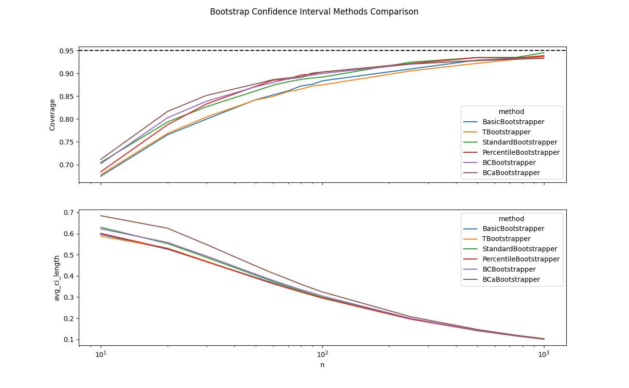
Next, I looked at a more complex statistic over a more complex distribution. This time the observed coverage was far less than that promised by the nominal rate for small $n$, with all methods starting at around $\approx 70\%$. Interestingly, the performance of each approach is roughly in line with the order that they were presented in my original exploration, with the difference in coverage between the worst and best performing methods being within $\approx 5\%$. Additionally, all methods did eventually converge to the nominal rate as $n \rightarrow \infty$.

    def complex_distribution(key: jax.Array, n: int) -> jax.Array:
        # Log-normal distribution (heavily skewed)
        key, subkey = random.split(key)
        log_normal = jnp.exp(random.normal(subkey, shape=(n,)))

        # Add some contamination for extra complexity
        key, subkey = random.split(key)
        contamination = random.exponential(subkey, shape=(n,))

        return 0.9 * log_normal + 0.1 * contamination

    def complex_statistic(data: jax.Array) -> jax.Array:
        return jnp.mean(data) / (1 + jnp.median(data))

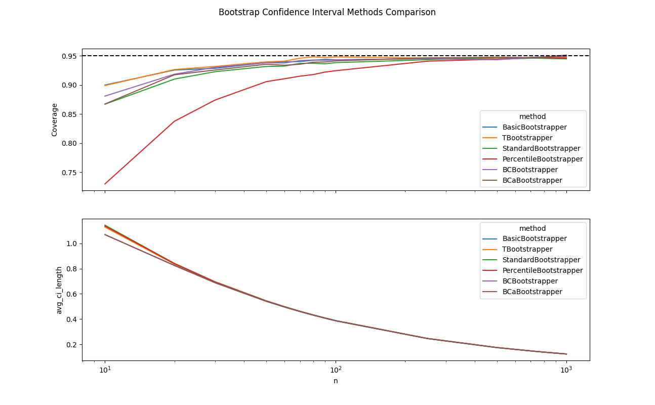
Adversarial Percentile Setup

Thus far, I was surprised to see that the percentile method was on par with the other more complex methods. After all, my original exploration set out to challenge my default approach of reaching for the percentile method. As such, I wanted to devise an adversarial example that the percentile method would struggle on. Specifically, I modified my bootstrap resampling code to add a constant offset, with scale set by the statistic variance (for the sake of numerical stability), to the estimated statistic and twice this offset to the replicates. This perturbation ensured that the difference between the estimators and true statistics would be offset by some constant amount. This is a scenario that the percentile method will struggle with, since its estimated percentiles will be off by twice this offset. Meanwhile, the other methods make pivotal assumptions about statistic differences and as such will be insulated from this perturbation.

\[\hat{\theta}_n - \theta \sim C + F\] \[\hat{\theta}^* - \hat{\theta} \sim C + F\]

def resample(self, data: jax.Array, n_resamples: int = 2000, key: jax.Array = random.key(42)) -> None:
    key, subkey = random.split(key)

    self._theta_hat = self._statistic(data)

    @jax.vmap
    @jax.jit
    def _generate_bootstrap_replicate(rng_key: jax.Array) -> jax.Array:
        data_resampled = self._resample_data(data, rng_key)
        theta_boot = self._statistic(data_resampled)
        return theta_boot

    self._bootstrap_replicates = _generate_bootstrap_replicate(random.split(subkey, n_resamples))

    # Modification
    bias_factor = self.variance() * 2
    self._theta_hat = self._theta_hat + bias_factor
    self._bootstrap_replicates = self._bootstrap_replicates + 2 * bias_factor

No Free Lunch

People often point to bootstrapping as an “assumption-free” panacea for confidence interval estimation in the age of computer-aided statistics. Hopefully, this analysis has shown that there is indeed a price for using bootstrap confidence interval estimation, namely that the true coverage can be considerably less than the nominal level, especially for $n \leq 100$. Furthermore, the success of different bootstrapping approaches, in terms of rapidly converging to their promised asymptotic results, very much depends on whether the supplied data conforms to that bootstrap method’s optimal convergence assumptions.

However, we should not be too harsh on bootstrapping. Classical statistics often makes equally dubious data generation and asymptotic assumptions. In summary, bootstrapping is a powerful tool; however, professional judgment should be exercised before blindly accepting the confidence intervals that these procedures produce. Furthermore, if you have good reason to believe that your data conforms to assumptions that would make it amenable to exact confidence interval calculation, then such procedures should not be overlooked.