Building An Autodiff Library

Introduction

Until recently, despite my extensive experience with auto-differentiation frameworks, I have never implemented one myself. I believe that implementing a tool that you commonly use yourself can yield great benefits regarding your intuition when using said tool. You stop having to memorise “patterns”, you simply start thinking about what needs to be done at a lower level and what the sensible higher level abstractions would be to facilitate this. This either triggers you to remember the “pattern”, or prompts you to search for sensible terms in the documentation. Furthermore, I would argue this is the same reason why being exposed to other framework/languages can strengthen your abilities in your current framework/language.

The Python Autodiff Landscape

I have been using automatic differentiation libraries in Python for over 5 years. I started this journey with the Keras API for TensorFlow, which provided high level abstractions to define basic layered neural networks. I then moved onto the TensorFlow Model and Functional APIs which allowed for a much higher degree of flexibility, namely I was able to define my own custom layers and functions. Furthermore, during my Masters dissertation I was exposed to TensorFlow Probability, which further extended my tool kit, allowing me to seamlessly define probabilistic models within deep learning frameworks.

Professionally, I now use a combination of PyTorch and JAX. From my experience, I believe the former excels in productionising fairly standard or established architectures, while the latter excels in research or high-performance computing contexts. I believe these differences primarily stem from the different programming paradigms they promote. PyTorch’s OOP approach leads to additional initial investment in terms of infrastructure, but ultimately leads to more extensible and maintainable code. Meanwhile, JAX’s lack of high-level abstractions actually frees you to tell the framework exactly what you want it to do. More specifically, you don’t have to worry about making your implementation conform to the set of abstractions/interfaces supplied by the framework, which is especially useful when you are implementing something novel. Although, it should be stressed that both frameworks are very well suited for any problems requiring automatic differentiation, and an expert in either framework is going to have no problem getting around the problems that are a little more awkward in that framework relative to the other.

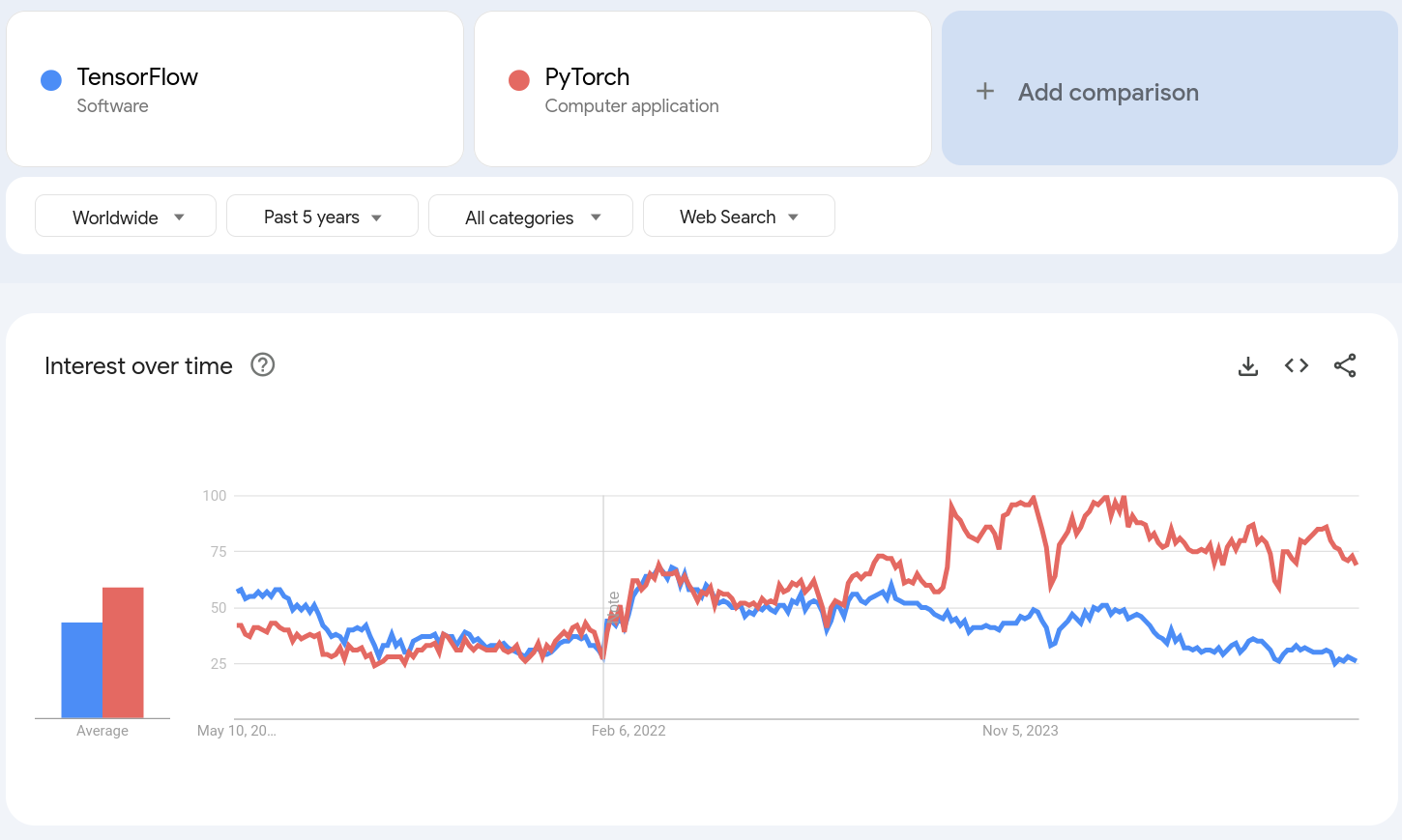
My move away from TensorFlow was motivated by my dissatisfaction in the large amount of boiler plate that it forced, and what in my opinion were non-sensible defaults (e.g. requiring context managers to track gradients, rather than context mangers to not track gradients). I do not seem to be alone in this switch. Indeed, google trends would suggest that TensorFlow was the dominant framework when I started learning about deep learning, but has been greatly surpassed by PyTorch in recent years.

Much of the strength of JAX lies in its Just In Time (JIT) compilation capabilities, which facilitate drastic performance improvements for frequently executed code. Development of such functionality is not of pedagogical interest for this project. I am not interested in building a high performance library, but rather deepening my intuition in automatic differentiation. Meanwhile, Pytorch’s higher compatibility for dynamic compute graphs is of pedagogical interest. Therefore, PyTorch will be the primary source of inspiration for this library.

Automatic Differentiation Recap

For a full discussion on automatic differentiation, see my original blog post, where I derived the equations for reverse mode automatic differentiation. To recap, for each vertex $v$ in our compute graph, we define the adjoint variable:

\[\bar{v}=\frac{\partial f}{\partial v} \quad \forall v \in V,\]

Where $f$ represents the output vertex of our compute graph. In the context of neural networks we can think of this as the scalar valued loss function that our network feeds into.

Furthermore, we derived the backward equations:

\[\bar{v} = \frac{\partial f}{\partial v} =\sum_{u \in \text{children}(v)}\frac{\partial f}{\partial u}\frac{\partial u}{\partial v} = \sum_{u \in \text{children}(v)}\bar{u}\frac{\partial u}{\partial v}\]

Which allow us to “back propagate” the adjoint values for children to their parents. When we pair this with the trivial end vertex evaluation $\bar{f}=1$ and pre-implemented functions for evaluations of the vertex derivatives, i.e.

\[\frac{\partial v}{\partial u} \quad u \in \text{parent}(v)\]

This then empowers us to get the derivatives of arbitrary vertices in our compute graph with respect to the output vertex. Importantly, this allows us to get the derivative of weights with respect to the loss in an efficient procedure of comparable computational complexity to the forward pass.

Implementation

We will now define the high level abstractions required to build an automatic differentiation framework. In the interest of brevity we will not detail the entire implementation for this project. However, the full source code can be found on my my GitHub

Vertex

The Vertex will serve as the fundamental data type for this project. Its core functionality will be to store a value and an adjoint value, i.e. grad. Furthermore, the backpropagation equation suggests that we calculate adjoint values for a vertex using the adjoint values from its children. Therefore, the most direct way to do this would be for vertices to store their children. However, from an implementation stand point, in terms of building dynamic compute graphs, this is quite un-natural. It is much more natural to add the parents of a vertex, i.e. its inputs, to this newly created vertex’s _parents attribute, than it is to go through each input and update its children. Furthermore, if we are going to back-propagate, we will need to perform some sort of graph traversal from parents to children, i.e. we are going to need these references anyway. Finally, we include an attribute _backward which will allow us to define the node wise derivative of the Vertex relative to its inputs/parents.

class Vertex:
    def __init__(
        self,
        value: float,
        _parents: tuple[Self, ...] | None = None,
        _backward: Callable[[tuple[Self, ...]], tuple[float, ...]] | None = None,
    ):
        self.value = value
        self.grad = 0

        # Implementation detials for backpropogation - _backward produces node wise gradients per _parent
        self._parents = tuple() if _parents is None else _parents
        self._backward = lambda *n: (0,) if _backward is None else _backward

    def __repr__(self) -> str:
        return f"{type(self).__name__}({repr(self.value)})"

The next step is going to be implementing backwards equations. Given a vertex $u$ and a parent $v$, then the contribution of $u$ to $v$’s adjoint value is exactly equal to: \(\frac{\partial f}{\partial u}\frac{\partial u}{\partial v}\) The above quantity can be calculated using all of the information contained in our Vertex class, i.e. the left value is self.grad and the right value is the result of self._backward(*self.parents). Therefore we can send a vertex’s contribution to its parents by iterating over its self._parents attribute.

The challenge here is that we need to be careful with the order in which we process vertices. If we send updates back for a given vertex before it has received all of its updates from its children, then the value it sends back via its self.grad won’t be accurate/complete. In other words we need to ensure that all children are processed before their parent.

In the language of graph theory, we would say that we require the vertices to be processed in a topologically sorted order. The algorithm for getting a valid topological sorting is to perform a post-order Depth First Search (DFS). Specifically, we add a vertex to the next available slot at the end of the topological sort, if and only if all of its children have been processed, i.e. are already ahead of it in the topological sort. In practice we simply append to a dynamic array and reverse it at the end to get the same effect. Finally, we keep track of all the nodes that we have processed (seen) such that we do not reprocess a node if we reach it through an alternative branch.

    def _get_topo_sort(self, topo_sort: list[Self], seen: set[Self]) -> None:
        seen.add(self)
        for parent in self._parents:
            if parent not in seen:
                parent._get_topo_sort(topo_sort=topo_sort, seen=seen)
        topo_sort.append(self)

    def get_topo_sort(self):
        topo_sort: list[Self] = []
        seen: set[Self] = set()

        self._get_topo_sort(topo_sort, seen)

        return topo_sort[::-1]

With a topological sorting of our compute graph defined we are now free to iterate through the nodes in topological order and send their gradient updates to their parents. As a final caveat, we set the initial adjoint value to 1 , due to this representing the output node’s adjoint value.

    def backward(self):
        # Set the top level node gradient to one, i.e. its gradient with respect to itself
        self.grad = 1

        # Send gradients back in topological order,
        # such that all children send gradients back before parent is processed
        topo_sort = self.get_topo_sort()
        for u in topo_sort:
            node_grads = u._backward(*u._parents)
            for v, node_grad in zip(u._parents, node_grads):
                v.grad += u.grad * node_grad

Finally, we need some way to reset our compute graph after we have used our calculated gradients for their desired purpose, e.g. an optimiser step/upate. This can be performed with a simple DFS on the vertices in the graph.

    def zero_grad(self):
        seen = set()

        def dfs(root: Self):
            root.grad = 0
            seen.add(root)

            for parent in root._parents:
                if parent not in seen:
                    dfs(parent)

        dfs(self)

Function

The next important abstraction is the function abstraction. This has two abstract methods, forward and backward. The former is used by the __call__ method to get the resulting output vertex for the forward compute of the function, and the latter is used to tack on the vertex wise derivative to this resulting output vertex.

class Function(ABC):
    @classmethod
    def __call__(cls, *args) -> "Vertex":
        z = cls.forward(*args)

        # Add parents and backwards function for backprop
        z._parents = args
        z._backward = cls.backward

        return z

    @staticmethod
    @abstractmethod
    def forward(*args) -> "Vertex":
        raise NotImplementedError

    @staticmethod
    @abstractmethod
    def backward(*args) -> tuple[float, ...]:
        raise NotImplementedError

For example, two of the most fundamental functions are add and mult, which can be implemented as follows:

class Add(Function):
    @staticmethod
    def forward(*args) -> Vertex:
        z = Vertex(sum(v.value for v in args))
        return z

    @staticmethod
    def backward(*args) -> tuple[float, ...]:
        return (1.0,) * len(args)


add = Add()


class Mult(Function):
    @staticmethod
    def forward(*args) -> Vertex:
        z = Vertex(prod(v.value for v in args))
        return z

    @staticmethod
    def backward(*args) -> tuple[float, ...]:
        n = len(args)

        pre = [1 for _ in range(n)]
        for i in range(1, n):
            pre[i] = args[i - 1].value * pre[i - 1]

        post = [1 for _ in range(n)]
        for i in range(n - 2, -1, -1):
            post[i] = args[i + 1].value * post[i + 1]

        return tuple(pre[i] * post[i] for i in range(n))


mult = Mult()

The above Function abstraction was used to define many functions for the library, including the typical dunder methods for the Vertex class. However, these details have been omitted for brevity.

Vector and Matrix

We now define a Vector and Matrix class. Again we omit the trivial dunder methods, but have shown how the dot product and matrix multiplication operations are defined in terms of our add and multiply function.

class Vector(Sequence):
    def __init__(self, *args):
        if len(args) == 0:
            raise ValueError("No data supplied.")

        if isinstance(args[0], Sequence):
            assert len(args) == 1, (
                "Constructor either takes vertices via variadic arguments, or an iterator."
            )
            parsed_args = list(args[0])
        else:
            parsed_args = list(args)

        for i in range(len(parsed_args)):
            if isinstance(parsed_args[i], Vertex):
                continue
            elif isinstance(parsed_args[i], float):
                parsed_args[i] = Vertex(parsed_args[i])
            else:
                raise ValueError(
                    "All passed arguments must be either of type Vertex or float."
                )

        self._data: tuple[Vertex, ...] = tuple(parsed_args)
 
    def __getitem__(self, item: int) -> Vertex:
        return self._data[item]

    def __len__(self) -> int:
        return len(self._data)

...

    def dot(self, other: Self) -> Vertex:
        return F.add(*(self * other))

class Matrix(Sequence):
    def __init__(self, data: Sequence[Sequence[float | Vertex]]):
        assert len(data) > 0, "At least one row of data must be supplied."
        m = len(data)

        cols = set()
        for r in range(m):
            cols.add(len(data[r]))
        assert len(cols) == 1, (
            f"Inconsistent column numbers in supplied data, n_cols: {cols}"
        )
        n = cols.pop()

        parsed = []
        for r in range(m):
            row = []
            for c in range(n):
                item = data[r][c]
                if isinstance(item, Vertex):
                    row.append(item)
                elif isinstance(item, float):
                    row.append(Vertex(item))
                else:
                    raise ValueError(
                        "All passed arguments must be either of type Vertex or float."
                    )
            parsed.append(row)

        self._rows: tuple[Vector, ...] = tuple(Vector(row) for row in parsed)
        self._cols: tuple[Vector, ...] = tuple(
            Vector(tuple(row[c] for row in parsed)) for c in range(n)
        )

    @overload
    def __getitem__(self, key: int) -> Vector: ...

    @overload
    def __getitem__(self, key: tuple[int, int]) -> Vertex: ...

    def __getitem__(self, key: int | tuple[int, int]) -> Vertex | Vector:
        if isinstance(key, tuple):
            assert len(key) == 2, "Tuple keys must have length 2."
            r, c = key
            return self._rows[r][c]
        elif not isinstance(key, float):
            return self._rows[key]
        else:
            raise ValueError("Key must be int or tuple of ints.")

    def __len__(self) -> int:
        return len(self._rows)

    @property
    def shape(self) -> tuple[int, int]:
        return len(self._rows), len(self._rows[0])

 ...
 
    @overload
    def __matmul__(self, other: Vector) -> Vector: ...

    @overload
    def __matmul__(self, other: Self) -> Self: ...

    def __matmul__(self, other: Self | Vector) -> Self | Vector:
        is_vec = isinstance(other, Vector)
        if is_vec:
            other = type(self)([[v] for v in other])

        n, k1 = self.shape
        k2, m = other.shape
        assert k1 == k2, f"Incompatible matrix multiplication dims {k1}!={k2}"

        out = []
        for r in range(n):
            row = []
            for c in range(m):
                row.append(self._rows[r].dot(other._cols[c]))
            out.append(row)

        if is_vec:
            return Vector([v[0] for v in out])

        return type(self)(out)

A reasonable extension at this point would be to define a general Tensor, but for this simple project I deemed the above as satisfactory.

Neural Networks

We now define an abstraction for neural network components, i.e. the Component class. Then we define a Linear layer and Sequential component which composes layers.

class Component(ABC):
    def __init__(self, *args, **kwargs) -> None:
        self._parameters = {}

    def __call__(self, x: Vector) -> Vector:
        return self.forward(x)

    @property
    def parameters(self) -> dict:
        return self._parameters

    @abstractmethod
    def forward(self, x: Vector) -> Vector:
        raise NotImplementedError

class Linear(Component):
    def __init__(
        self,
        in_dim,
        out_dim,
        bias: bool = True,
        activation: Function | None = None,
        weight_initialiser: WeightInitialiser = He(),
        seed: int = 42,
    ) -> None:
        super().__init__()

        random.seed(seed)
        W = Matrix(
            [
                [random.gauss(0, math.sqrt(2 / in_dim)) for _ in range(in_dim)]
                for _ in range(out_dim)
            ]
        )
        weight_initialiser(W)
        self._parameters["W"] = W

        if bias:
            self._parameters["b"] = Vector([0.0 for _ in range(out_dim)])

        self._activation = activation

    def forward(self, x: Vector) -> Vector:
        z = self.parameters["W"] @ x
        z = typing.cast(Vector, z)

        if "b" in self.parameters:
            z = z + self.parameters["b"]

        if self._activation is not None:
            z = Vector([self._activation(v) for v in z])

class Sequential(Component):
    def __init__(self, layers: list[Component]) -> None:
        super().__init__()
        self._layers = layers
        for i, layer in enumerate(layers):
            self._parameters[str(i)] = layer._parameters

    def forward(self, x: Vector) -> Vector:
        z = x
        for layer in self._layers:
            z = layer(z)
        return z

For brevity we will not go into detail on the initialisers or optimisers for Component instances. The latter simply takes in a set of component parameters, which can be nested in nature, and initialises a set of optimisation parameters per learnable parameter. This then allows for general optimisation methods like Adam to be implemented. During an optimiser step the parameter tree and optimisation parameters tree are traversed together in order to make gradient based updates using both the parameter’s gradient and its optimisation parameters.

End-to-End Tests

Linear Data Generation Process

As a first test we fit a Linear layer to a linear data generation process and see how well it fits the parameters.

def linear_data_gen_experiment():
    """
    Run an experiment to fit a linear model to synthetically generated linear data.

    This function:
    1. Generates random linear data with noise
    2. Creates a linear model
    3. Trains the model using Adam optimizer
    4. Prints the loss for each epoch
    5. Compares the true parameters with the learned parameters
    """
    random.seed(42)
    m = 5
    n = 10_000
    X = Matrix([[random.uniform(-1, 1) for _ in range(m)] for _ in range(n)])

    beta = Vector([random.gauss(-1, 1) for _ in range(m)])
    noise = Vector([random.gauss(0, 0.1) for _ in range(n)])
    y = X @ beta + noise

    model = Sequential([Linear(m, 1, bias=False)])

    opt = MomentumSGD(model.parameters, nu=0.01, momentum=0.9)

    epochs = 100
    for i in range(1, epochs + 1):
        loss_total = 0
        for j in range(n):
            pred_j = model(X[j])[0]
            loss = loss_fn(pred_j, y[j])
            loss = loss / n
            loss_total += loss.value

            loss.backward()
            opt.step()
            loss.zero_grad()

        print(f"{i} / {epochs} - {loss_total=}")

    print("True Parameter - Learned Parameter")
    for true_param, learned_param in zip(beta, model.parameters["0"]["W"][0]):
        print(f"{true_param} - {learned_param}")

This resulted in the output below, which shows the model successfully learned the correct parameters.

True Parameter - Learned Parameter
Vertex(0.44661426582452757) - Vertex(0.4462050447411561)
Vertex(-1.3078976781240659) - Vertex(-1.30579607982552)
Vertex(-0.404920714804475) - Vertex(-0.4046215004941457)
Vertex(0.3689330136599842) - Vertex(0.36713642387257217)
Vertex(-0.560598703419118) - Vertex(-0.5597352938168645)

Non-Linear Data Generation Process

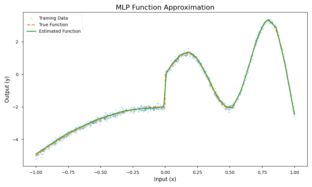
As a more difficult test we will now fit a single input non-linear data generation process using a 10 layer neural network.

def non_linear_data_gen_experiment():
    """
    Run an experiment to fit a deep neural network to synthetically generated non-linear data.

    This function:
    1. Generates random non-linear data with noise using a piecewise function
    2. Creates a deep neural network with multiple relu activation layers
    3. Trains the model using Adam optimizer
    4. Prints the loss for each epoch
    5. Visualizes the true function, training data, and model predictions
    """
    random.seed(42)
    n = 1000
    X = Matrix([[random.uniform(-1, 1)] for i in range(n)])

    def f(X: float) -> float:
        if X < 0:
            return -3 * (X**2) - 2
        else:
            return math.exp(1.5 * X) * math.sin(10 * X)

    y = Vector([f(X[i][0].value) for i in range(n)])
    noise = Vector([random.gauss(0, 0.1) for _ in range(n)])
    y = y + noise

    h = 10
    model = Sequential(
        [
            Linear(1, h, activation=relu, weight_initialiser=He(), seed=1),
            Linear(h, h, activation=relu, weight_initialiser=He(), seed=2),
            Linear(h, h, activation=relu, weight_initialiser=He(), seed=3),
            Linear(h, h, activation=relu, weight_initialiser=He(), seed=4),
            Linear(h, h, activation=relu, weight_initialiser=He(), seed=5),
            Linear(h, h, activation=relu, weight_initialiser=He(), seed=6),
            Linear(h, h, activation=relu, weight_initialiser=He(), seed=7),
            Linear(h, h, activation=relu, weight_initialiser=He(), seed=8),
            Linear(h, h, activation=relu, weight_initialiser=He(), seed=9),
            Linear(h, 1, seed=5),
        ]
    )

    opt = Adam(model.parameters, nu=0.001, beta_1=0.9, beta_2=0.999)

    epochs = 100
    for i in range(1, epochs + 1):
        loss_total = 0
        for j in range(n):
            pred_j = model(X[j])[0]
            loss = loss_fn(pred_j, y[j])
            loss = loss / n
            loss_total += loss.value

            loss.backward()
            opt.step()
            loss.zero_grad()

        print(f"{i} / {epochs} - {loss_total=}")

The result of the fitting procedure is shown below. The fitted function (green) closely matches the true data generation process (orange).