A Deep Dive On Vanishing And Exploding Gradients

Introduction

I was first introduced to the vanishing/exploding gradients problem while conducting my Bachelor’s thesis. At the time I was reading the textbook “Hands-On Machine Learning with Scikit-Learn and TensorFlow”. The textbook warned against using naive weight initialisation schemes such as using a standard normal. Instead they prescribed that you use “Glorot” for saturating activations, “He” for ReLU variants, and “LeCun” for SELU dense networks. The book gave intuitive arguments for these initialisation schemes, and pointed the reader to the original papers for full mathematical details.

At the time, I found the arguments in the textbook convincing enough, and as such I did not read the original papers. I don’t necessarily regret this decision, my thesis was first and foremost on quantum mechanics, deep learning was just a tool I was using at the time. However, what I do regret, is not going back and reading these papers at a later date. The modern success of deep neural networks would not be possible if it wasn’t for the progress made on the vanishing gradients issue in the 2010s. In fact, before this problem was solved interest in deep learning had drastically diminished by the early 2000s, with many believing that training deep neural networks simply wasn’t feasible.

Weight Initialisation

Symmetry Breaking

One key consideration is that of symmetry breaking. For example, if all parameters were initialised with the same values then all the pre-activations for the first layer would be the same, which would lead to all the same pre-activations in the next layer, …, the result is that each parameter in a given layer has the exact same effect on the loss function and as such gradient updates are identical. This means that the model is unable to break free from this symmetry. One way to achieve symmetry breaking is by randomly generating parameters, usually either some form of Gaussian or uniform distribution

Expectation Considerations

parameter distributions are usually set to have a mean of zero, this is because a non-zero mean could accumulate during forward propagation and cause saturation in later layers, which would exacerbate the vanishing/exploding gradients. However, when dealing with non-saturating activations such as the ReLU activation, then this saturating problem is less of an issue, and some argue that the biases should be set to a small non-zero value to encourage neurons to be “turned-on” during initialisation.

Variance Considerations

There are a number of different approaches for initialising the variance, their differences stem from the different aspects of our network that they are trying to stabilise.

In the following sections we will assume that we have chosen an activation function such that $\phi^{(l)’}(0) = 1$ and that our post-activation stabilisation procedure is working, meaning that our pre-activations are relatively small. This will then let us use a zeroth order approximation $\phi^{(l)’}(a^{(l)}) \approx 1$. Importantly, since we are assuming the thing we are analysing, the conditions that these analyses will produce will be necessary conditions for stability, i.e. conditions which when not upheld imply that the quantity of interest is not stable. However, the converse is not necessarily true, i.e. our approximation could be poor, rendering the analysis invalid.

Additionally, it should be stressed that the following probabilistic analyses are based purely on the initialisation of the network, i.e. they are making no statement about the variance of the trained network, simply the properties associated with the random process of initialisation. Therefore, we will be analysing necessary conditions for initial stability. Heuristically, this is of interest since it is unlikely that an unstable initialisation will suddenly stabilise during training, i.e. we don’t want to set our optimisation up to fail.

Post-Activation Stability

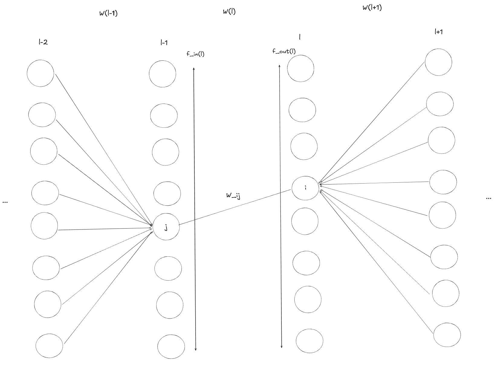
The Multilayer Perceptron (MLP) forward equations are:

\[a^{(l)} = W^{(l)}h^{(l-1)} + b^{(l)}\] \[h^{(l)} = \phi^{(l)}(a^{(l)})\]

First, due to the fact that biases are set to a constant value of zero, or something close to it, they do not contribute to the variance. This means that:

\[\mathbb{V}(a^{(l)}_i) = \mathbb{V}\left(\sum_jW^{(l)}_{ij}h^{(l-1)}_j + b^{(l)}_i\right) = \mathbb{V}\left(\sum_{j}W_{ij}^{(l)}h_j^{(l-1)}\right)\]

We now assume that the weights are independently and identically distributed, and that their initialisation does not depend on the data, i.e. pre-activations.

\[\mathbb{V}(a^{(l)}_i) = \sum_{j}\mathbb{V}\left(W_{ij}^{(l)}\right)\mathbb{V}\left(h_j^{(l-1)}\right) = \mathbb{V}(w_i) \sum_{j}\mathbb{V}\left(h_j^{(l-1)}\right)\]

Now to get the variance of the post-activation we use the delta method, which is valid via the CLT since we are dealing with large sums of random variables.

\[\mathbb{V}(h^{(l)}_i) = \phi^{(l)'}(a^{(l)})\mathbb{V}(a^{(l)}_i)\]

We now assume we have chosen an activation function such that $\phi^{(l)’}(0) = 1$ and that our post-activation stabilisation procedure is working, meaning that our pre-activations are stable and relatively small. Therefore, we can make the zeroth order approximation $\phi^{(l)’}(a^{(l)}) \approx 1$, which leads to:

\[\mathbb{V}(h^{(l)}_i) = \mathbb{V}(w_i^{(l)}) \sum_{j}\mathbb{V}\left(h_j^{(l-1)}\right)\]

We now draw attention to the base case of $\mathbb{V}(h^{(0)}_i)=\mathbb{V}(x)$, where we assume all input features have the same variance. If we call the number of summands in each of the above sums the “fan-in” $f_{in}$, i.e. the dimensionality that $W^{(l)}$ maps from. Then it is easy to show using induction that:

\[\mathbb{V}(h^{(l)}_i) = \mathbb{V}\left(x\right)\prod_{l'=1}^{l} f_{in}^{(l')}\mathbb{V}(w^{(l')})\]

Therefore, if we want our forwards pass to be stable, i.e. $\mathbb{V}(h^{(l)})=\mathbb{V}(h^{(l’)}) \ \forall l, l’$, then the above equation implies that we need

\[\mathbb{V}(w^{(l)})=\frac{1}{f_{in}^{(l)}} \quad \forall l\]

Making our derivations in terms of “number of summands”, i.e. fan-in, is beneficial because the analysis generalises beyond dense neural networks. For example, to apply the above analysis to a 2D convolutional neural network the “fan_in” is the total kernel area multiplied by the number of input channels, for example this could be $f_{in}=W\times H \times C = 3\times 3 \times 8$.

Node Sensitivity Stability

The backward equations for an MLP are given below.

\[\frac{\partial E}{\partial a^{(l)}_i} = \phi'(a^{(l)})\sum_{j} (W^{(l+1)})^T_{ij} \frac{\partial E}{\partial a^{(l+1)}_j}\]

Suppose we have a $L$ layer neural network. Then, if we again assume that we are in a linear activation function regime and that the weights of a given layer are independently and identically distributed then it follows that

\[\mathbb{V}\left(\frac{\partial E}{\partial a^{(l)}_i}\right) = \mathbb{V}(w^{(l+1)}) \sum_{j} \mathbb{V}\left(\frac{\partial E}{\partial a^{(l+1)}_j}\right)\]

Again, if we start with the base case that $\mathbb{V}\left(\frac{\partial E}{\partial a^{(L)}_j}\right)$ are all equal, then it can be shown with induction that

\[\mathbb{V}\left(\frac{\partial E}{\partial a^{(l)}_i}\right) = \mathbb{V}\left(\frac{\partial E}{\partial a^{(L)}_j}\right) \prod_{l'=l+1}^L f_{out}^{(l')}\mathbb{V}(w^{(l')})\]

Where “fan-out” $f_{out}^{(l)}$ is equal to the dimensionality of the space that $W^{(l)}$ maps to.

Therefore, if we want our backwards pass to be stable, i.e. $\mathbb{V}\left(\frac{\partial E}{\partial a^{(l)}}\right) = \mathbb{V}\left(\frac{\partial E}{\partial a^{(l’)}}\right) \ \forall l, l’$, then the above equation implies that we need

\[\mathbb{V}(w^{(l)})=\frac{1}{f_{out}^{(l)}} \quad \forall l\]

Gradient Stability

We now recall the link between node sensitivities and weight gradients.

\[\frac{\partial E}{\partial W^{(l)}_{ij}}= \frac{\partial E}{\partial a_i^{(l)}} h_j^{(l-1)}\]

Importantly, this means that

\[\mathbb{V}\left(\frac{\partial E}{\partial W^{(l)}_{ij}}\right)= \mathbb{V}\left(\frac{\partial E}{\partial a_i^{(l)}}\right) \mathbb{V}\left(h_j^{(l-1)}\right)\]

The previous analyses gave us expressions for the variances of the post-activations and node sensitives, which can now be substituted into the above equation.

\[\mathbb{V}\left(\frac{\partial E}{\partial W^{(l)}_{ij}}\right) = \left(\prod_{l'=1}^{l-1} f_{in}^{(l')}\mathbb{V}(w^{(l')})\right) \left(\prod_{l'=l+1}^L f_{out}^{(l')}\mathbb{V}(w^{(l')})\right)\mathbb{V}\left(x\right)\mathbb{V}\left(\frac{\partial E}{\partial a^{(L)}_j}\right)\]

I believe this actually deviates slightly from the equation given by Glorot et al., which includes the variances for the weights of every layer in the network, including layer $l$. I believe they made a mistake when moving from equation (2) to equation (6) in their paper. Equation (2) would indicate, that after assuming a linear regime, $l+1$ terms are the smallest terms that can appear, further expansions only lead to larger layer terms. Intuitively this makes sense, when we draw the compute graph, the current layer cannot contribute any “compounding factors”, i.e. $f_{out}^{(l)}\mathbb{v}(w^{(l)})$ does not belong in the above equation.

Now if we want our gradients to be stable, which is of key interest for the vanishing/exploding gradients problem, then we need:

\[\mathbb{V}(w^{(l)})=\frac{1}{f_{out}^{(l)}} \quad \forall l\] \[\mathbb{V}(w^{(l)})=\frac{1}{f_{in}^{(l)}} \quad \forall l\]

Importantly, if $f^{(l)}_{in} \neq f^{(l)}_{out}$, then it is not possible to simultaneously satisfy both of these equations. Which could explain the historic popularity of networks that utilise a constant number of hidden nodes per layer.

Furthermore, the above illustrates the importance of normalising your data. Input normalisation directly affects gradient variance via the multiplicative factor $\mathbb{V}(x)$. Meanwhile, output normalisation indirectly affects the gradient variance via the multiplicative factor $\mathbb{V}\left(\frac{\partial E(y, \hat{y})}{\partial a^{(L)}_j}\right)$.

Weight Initialisation Schemes

The above has built sufficient context for us to define different initialisation schemes.

LeCun

In 1998 Yann LeCun shared a “trick” for stabilising the signals in the forward pass of a MLP, the idea was to target a stable post-activation variance, to achieve this he advocated for using a weight distribution standard deviation of:

\[\sigma_w = \sqrt{\frac{1}{f_{in}}}\]

Which gives rise to the following uniform and normal initialisation distributions.

\[w \sim N\left(0, \frac{1}{f_{in}}\right)\] \[w \sim U\left(-\sqrt{\frac{3}{f_{in}}}, -\sqrt{\frac{3}{f_{in}}}\right)\]

Glorot

In 2010 Xavier Glorot and Yoshua Bengio were the first to come up with the probabilistic analysis detailed above, importantly, they showed that in order to have stable gradients, you needed to both stabilise the forward and the reverse pass.

However, as detailed above, if $f_{in}\neq f_{out}$ then this isn’t generally possible. Instead, they heuristically argued for a compromise, whereby we use $f_{avg}=\frac{f_{in}+f_{out}}{2}$ in place of $f_{in}$ for LeCun initialisation. This leads to a weight standard deviation of:

\[\sigma_w = \sqrt{\frac{2}{f_{in}+f_{out}}} = \sqrt{\frac{1}{f_{avg}}}\]

The resulting initialisation distributions for uniform and normal distributions are:

\[w \sim N\left(0, \frac{1}{f_{avg}}\right)\] \[w \sim U\left(-\sqrt{\frac{3}{f_{avg}}}, -\sqrt{\frac{3}{f_{avg}}}\right)\]

In their original paper they compare their initialisation directly against the “commonly used heuristic”:

\[w \sim U\left(-\sqrt{\frac{1}{f_{avg}}}, -\sqrt{\frac{1}{f_{avg}}}\right)\]

and showed that their approach was superior. Importantly, this is not LeCun initialisation, and this paper did not show Glorot initialisation to be superior or inferior relative to LeCun initialisation.

He

In 2015 He et al. argued that the “compromise” of Glorot initialisation was unnecessary. When using Glorot initialisation, we have:

\[\mathbb{V}(w^{(l')})=\frac{1}{f_{avg}}\]

Which, when plugged into our gradient variance equation, leads to a “instability factor” equal to:

\[\left(\prod_{l'=1}^{l-1} \frac{f_{in}^{(l')}}{f^{(l')}_{avg}}\right)\left(\prod_{l'=l+1}^L \frac{f_{out}^{(l')}}{f^{(l')}_{avg}}\right)\]

Which is a multiplication of $L-1$ terms, which have heuristically been argued to be close to 1, but are not necessarily equal to 1. Without further arguments, there is a concern that such a term will vanish/explode as the depth of the network is increased.

He et al. pointed out that it is sufficient to simply tackle one of the two stability conditions, since this mitigates the effect of the other. To see this, suppose we satisfy post-activation stability, then this would lead to:

\[\left(\prod_{l'=1}^{l-1} \frac{f_{in}^{(l')}}{f^{(l')}_{in}}\right) \left(\prod_{l'=l+1}^L \frac{f_{out}^{(l')}}{f^{(l')}_{in}}\right)= \left(\prod_{l'=l+1}^L \frac{f_{out}^{(l')}}{f^{(l')}_{in}}\right) = \frac{f_{out}^{(L)}}{f^{(l+1)}_{in}}\]

Conversely, if we satisfied node sensitivity stability, then this would lead to:

\[\left(\prod_{l'=1}^{l-1} \frac{f_{in}^{(l')}}{f^{(l')}_{out}}\right) \left(\prod_{l'=l+1}^L \frac{f_{out}^{(l')}}{f^{(l')}_{out}}\right)= \left(\prod_{l'=1}^{l-1} \frac{f_{in}^{(l')}}{f^{(l')}_{out}}\right) = \frac{f_{in}^{(1)}}{f^{(l-1)}_{out}}\]

Where we have used the fact that adjacent layers fan-in and fan-outs will cancel.

Importantly, the above “instability” factors have no potential for growing exponentially with depth. Their effect is completely controlled by the ratio of the fan-in/fan-out of input/output layers relative to some intermediate layer. Interestingly, this result would also seem to remove theoretical basis for preferring Glorot initialisation relative to LeCun initialisation.

Furthermore, He et al. adapted the original probabilistic analysis to the ReLU activation. The key idea, was that when we account for approximately half of the ReLUs “dying”, the result is that $f_{in}$ effectively reduces by a factor of 2. Furthermore, after accounting for the negative region of the ReLU via the reduction factor of 2, they did not have to assume a linear zeroth order approximation, i.e. the ReLU is linear with gradient 1 in the positive region. Importantly, this means that the stability analysis is both sufficient and necessary, which means that we can be certain that initialising our network in this way when using ReLU activations will lead to a stable initialisation.

To summarise, He initialisation advocates for satisfying only one of our original stability conditions, conventionally usually the forward pass condition, and it accounts for dying ReLUs by dividing $f_{in}$ by 2. This leads to a target standard deviation of:

\[\sigma_w = \sqrt{\frac{2}{f_{in}}}\]

The associated normal and uniform sampling distributions are:

\[w \sim N\left(0, \frac{2}{f_{in}}\right)\] \[w \sim U\left(-\sqrt{\frac{6}{f_{in}}}, -\sqrt{\frac{6}{f_{in}}}\right)\]

Experiments

I have found it hard to find direct comparisons of the above initialisation schemes. Indeed, from my initial introduction on this subject from “Hands-On Machine Learning with Scikit-Learn and TensorFlow” I was prescribed to use Glorot for saturating activations rather than LeCun. However, if the arguments presented by He. et al hold true for ReLUs then they should also hold true for saturating activations, i.e. Glorot has no theoretical reason to be superior to LeCun. I find this fascinating since the Glorot initialisation scheme is given a lot of credit for reigniting interest in deep learning in the 2010s, yet LeCun initialisation was known about all the way back in 1998. Furthermore, in the Glorot et al. paper the “commonly used heuristic” they compare their method against is not LeCun initialisation. This could indicate that LeCun initialisation unfortunately did not gain the traction it potentially deserved. This is especially tragic since had this method been widely adopted, we might have seen more interest in deep learning during the 2000s and could have had an extra decade of research to show for it.

The experiments below are performed on a “contracting pyramid” shaped network which contracts the number of hidden nodes by $4\%$ each layer. When accounting for floor division, this leads to a starting number of nodes of $1000$ to contract to $5$ after 100 layers. Finally a linear output layer of size $1$ is added to the network. This scalar output will act as the target of backpropogation, rather than the output of a loss function. The code for this is listed below.

def get_pyramid_model(
    n_layers: int = 1000,
    hidden_start: int = 100,
    ratio: float = 0.96,
    activation_fn: nn.Module = nn.ReLU(),
):
    # Add hidden layers
    layers = []
    n_hidden_prev = hidden_start
    for _ in range(n_layers):
        n_hidden = int(n_hidden_prev * ratio)

        layers.append(nn.Linear(n_hidden_prev, n_hidden))
        layers.append(activation_fn)

        n_hidden_prev = n_hidden

    # Add output layer
    layers.append(nn.Linear(n_hidden_prev, 1))

    model = nn.Sequential(*layers)

    return model

During the experiments I attached forward and backward “hooks” to the linear layers of the model such that their post-activations and sensitivities can be recorded.

    # Add tracking for intermediate forward and backward pass.
    forwards_record = []
    backwards_record = []
    for i, m in enumerate(model.modules()):
        if type(m) is nn.Linear:
            m.register_backward_hook(
                lambda module, backward_input, backward_output: backwards_record.append(
                    backward_output[0]
                )
            )
        elif type(m) is nn.ReLU or type(m) is nn.Sigmoid or type(m) is nn.Tanh:
            m.register_forward_hook(
                lambda module, forward_input, forward_output: forwards_record.append(
                    forward_output
                )
            )

Finally I took the standard deviations of these values and the weight gradients on a layer by layer basis. The final layer was ignored since its single observation does not give a reasonable estimate for the standard deviation. Furthermore, the backwards_record was reversed since it was appended to in reverse order during backpropagation. Finally, a stability value of eps=1e-12 was added to all values such that they can be plotted on a logarithmic scale without issues regarding negative infinities. Furthermore, if any values approached this value, then it was understood that this implied that the gradients were/had vanished.

    eps = 1e-12
    foward_stds = [np.std(f.detach().numpy()) + eps for f in forwards_record][:-1]
    backward_stds = [
        np.std(b.detach().numpy()) + eps for b in reversed(backwards_record)
    ][:-1]
    grad_stds = [
        np.std(m.weight.grad.numpy()) + eps
        for m in model.modules()
        if type(m) is nn.Linear
    ][:-1]

Shallow Saturating

The first experiment involved a naive initialisation which does not account for fan-in/fan-out, LeCun initialisation and Glorot initialisation. These initialisation methods were originally developed for shallow neural networks and as such I applied them to a 10 layer contracting pyramid network using a hyperbolic tangent activation.

def naive_uniform_init(m: nn.Module):
    with torch.no_grad():
        if type(m) is nn.Linear:
            weight = m.weight
            nn.init.uniform_(weight, -1, 1)
            nn.init.zeros_(m.bias)

def lecun_uniform_init(m: nn.Module):
    with torch.no_grad():
        if type(m) is nn.Linear:
            weight = m.weight
            f_out, f_in = weight.shape
            limit = math.sqrt(3 / f_in)
            nn.init.uniform_(weight, -limit, limit)
            nn.init.zeros_(m.bias)

def glorot_uniform_init(m: nn.Module):
    with torch.no_grad():
        if type(m) is nn.Linear:
            weight = m.weight
            f_out, f_in = weight.shape
            limit = math.sqrt(6 / (f_in + f_out))
            nn.init.uniform_(weight, -limit, limit)
            nn.init.zeros_(m.bias)

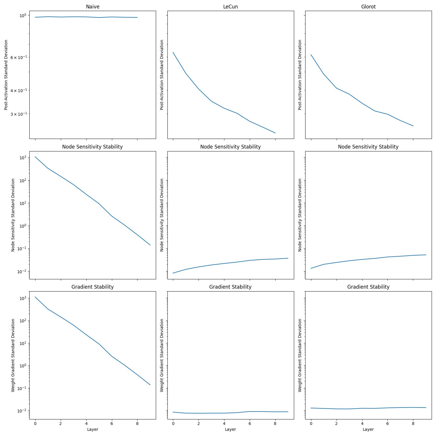
The naive initialisation led to gradient variances that span several orders of magnitude, while both LeCun and Glorot initialisation manage to maintain a consistent gradient variance. Furthermore, the naive post-activation variance converged to 1, which indicates that all the neurons saturated.

Deep Saturating

The previous analysis failed to show Glorot as superior to LeCun. I decided to repeat the analysis with 100 layers to see if Glorot helps train deeper saturating networks compared to LeCun.

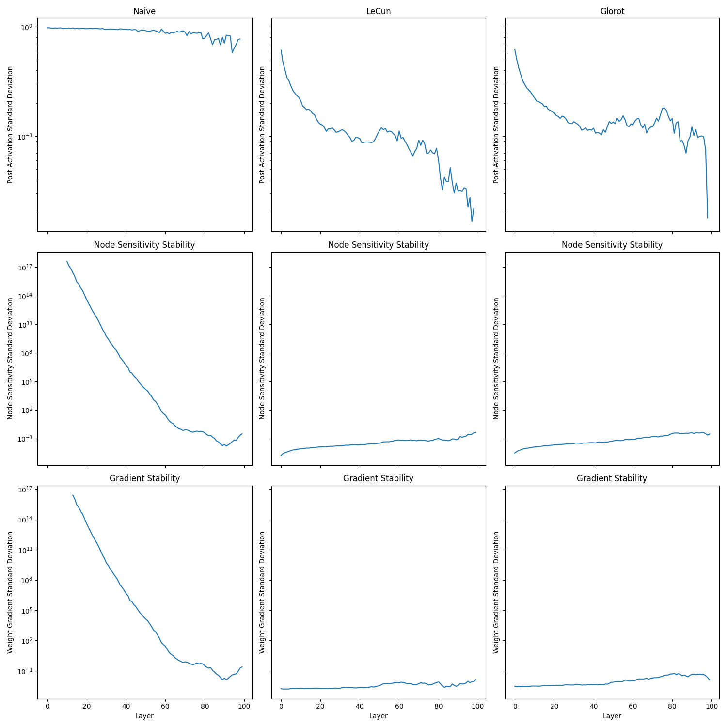
Again, both Glorot and Lecun where able to stabilise the network.

Deep Non-Saturating - Bad Initialisation

Next I swapped the activation function for a ReLU activation. The arguments from He et al. would imply that this should lead to instability across all previous strategies due to the dying ReLU problem.

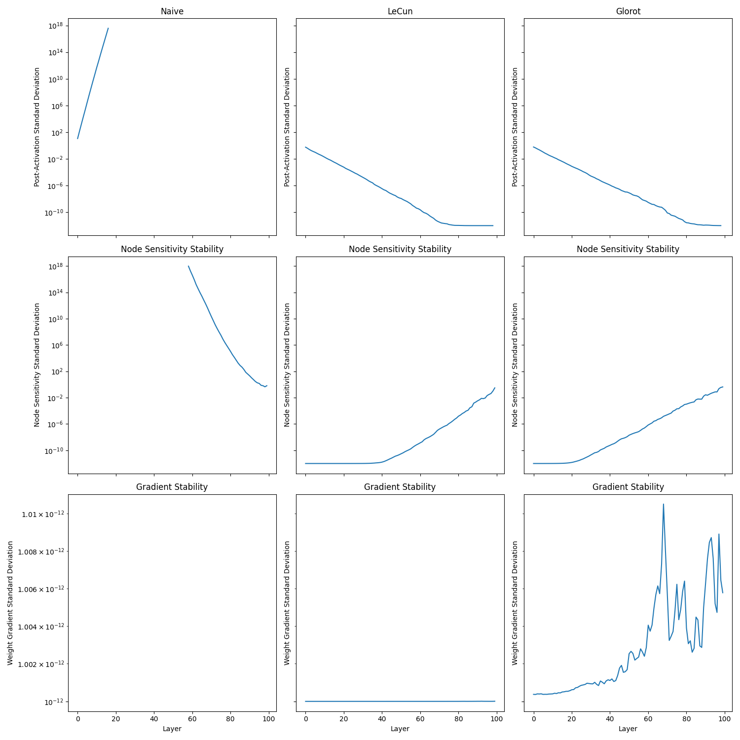
Indeed, the naive method suffered from exploding gradients, so much so that it overflows. Meanwhile LeCun and Glorot suffered from vanishing gradients, both approached the experiment’s minimum value of $10^{-12}$ .

Deep Non-Saturating

In the He et al. paper they state that using $f_{avg}$ is not necessary, and indeed the previous experiments were consistent with this conclusion. However, for completeness I added a variation of He initialisation that using $f_{avg}$.

def he_forward_uniform_init(m: nn.Module):
    with torch.no_grad():
        if type(m) is nn.Linear:
            weight = m.weight
            f_out, f_in = weight.shape
            limit = math.sqrt(6 / f_in)
            nn.init.uniform_(weight, -limit, limit)
            nn.init.zeros_(m.bias)


def he_backward_uniform_init(m: nn.Module):
    with torch.no_grad():
        if type(m) is nn.Linear:
            weight = m.weight
            f_out, f_in = weight.shape
            limit = math.sqrt(6 / f_out)
            nn.init.uniform_(weight, -limit, limit)
            nn.init.zeros_(m.bias)


def he_compromise_uniform_init(m: nn.Module) -> None:
    with torch.no_grad():
        if type(m) is nn.Linear:
            weight = m.weight
            f_out, f_in = weight.shape
            limit = math.sqrt(12 / (f_in + f_out))
            nn.init.uniform_(weight, -limit, limit)
            nn.init.zeros_(m.bias)

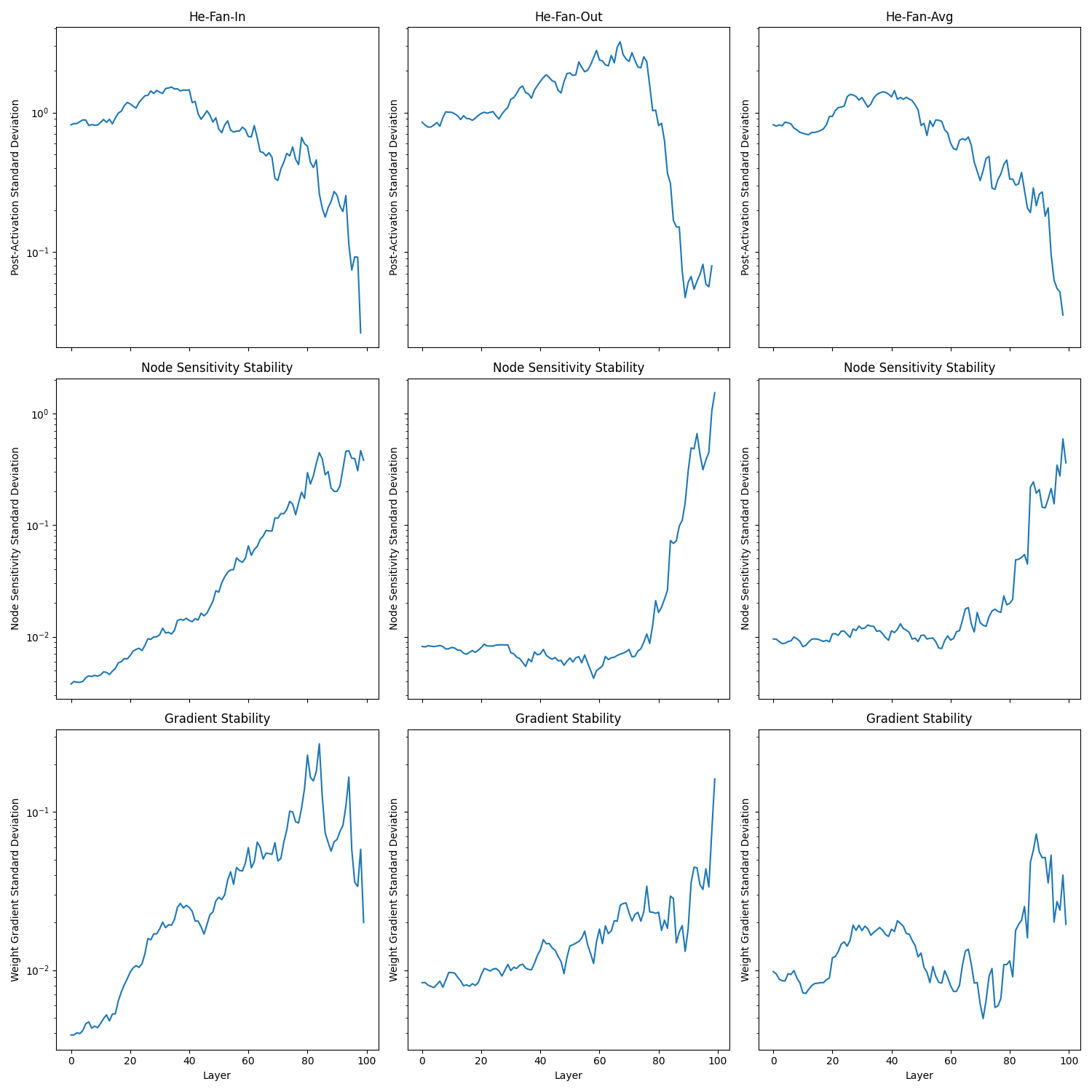
All 3 variations manged to stabilise the gradients and span around 3 orders of magnitude, which is exactly what is predicted by He et al. when having a $f_{in}^{(1)}=1000$ and $f_{out}^{(L)}=1$.

Batch Normalisation

As discussed, weight initialisation makes sure that gradients are stable during the beginning of training. However, it does not guarantee that they remain stable throughout. Unfortunately, a decent number of our probabilistic assumptions in our weight initialisation analysis are invalidated once we start training. For example, we can no longer assume weights are independent from each other, nor can we assume that the weights are independent of the data, in fact the reality is quite the contrary if our learning algorithm is working.

Fortunately, some important principles do carry forward. Namely, we have the issue that the gradient of a given node depends on all preceding post-activations and all proceeding node sensitivities. Which is unfortunately the recipe for issues regarding vanishing/exploding gradients due to multiplicative effects compounding. Another key insight that we can carry forward from our initialisation analysis is that it is sufficient to tackle post-activation stability, since if our post-activations are on a stable scale this also stabilises the scale of the gradients associated with those post-activations, which then indirectly stabilises the node sensitivity. However, one key difference relative to our previous analysis, is that we relax our goal of constant variance, we are okay with the network increasing the importance/scale of some layers relative to others during training, we simply do not want gradients to explode or vanish exponentially.

Batch normalisation attempts to tackle the above issues, it can be seen as an additional post-processing step performed directly on post-activations. During mini-batch gradient descent, we make mean $\mu_B$ and standard deviation $\sigma_B$ estimates over the post-activation values for that batch. This then allows us to normalise the post-activations to have a mean of zero and variance of 1. We then apply some learnable scale $\gamma$ and shift $\beta$ transformation to normalised post-activations. The entire procedure is detailed below:

1. $\mu_B = \frac{1}{m_B}\sum_{i=1}^{m_B}x^{(i)}$
2. $\sigma^2_B = \frac{1}{m_B}\sum_{i=1}^{m_B}(x^{(i)}-\mu_B)^2$
3. $\hat{x}^{(i)} = \frac{x^{(i)} - \mu_B}{\sqrt{\sigma_B^2 + \epsilon}}$
4. $z^{(i)} = \gamma \otimes \hat{x}^{(i)}+\beta$

It is more common to estimate the batch mean and batch standard deviation over the entirety of training using an exponentially weighted moving average, weighting more recent values higher. This allows you to freeze these estimates at the end of training such that they can be used during inference.

It might seem counterproductive to normalise the data and then introduce scale and shift parameters. However, if we do not allow the layer to learn a shift and scale, then we will have reduced the effective model capacity, this is obvious from the fact that the model could previously produce arbitrary intermediate post-activation distributions, but is now limited to mean zero variance one distributions. Importantly, there are now regular checkpoints in the compute graph which have their variance reset to one, which nullifies the effect of exploding/vanishing gradients.

The power in the above procedure is that it has decoupled the estimation of the scale and shift parameters, associated with some post-activation distribution, from the previous nodes in the neural network. This is actually the leading motivation for batch normalisation, not mitigating the vanishing/exploding gradients problem. This de-coupling drastically reduces the risk of “internal covariate shift” where small upstream changes have large effects on downstream post-activation distributions. Such shifts often disrupt training since the features that have been learned down-stream given some distribution over an intermediate representation might not be effective over the new intermediate representation distribution.

At inference time it is common to fuse the batch normalisation operation with the next layer’s matrix multiplication such that they can be performed as a single matrix multiplication, this means using batch normalisation is “free” in terms of performance at inference time.

Summary

• Normalise your data - the variance of your inputs sets the scale for post-activation variances and the variance of your outputs indirectly sets the scale for node-sensitivity variances.
• Use a weight initialisation scheme - The results of my experiments seem to indicate that stability is relatively agnostic relative to the choice of normalising factor, i.e. $f_{in}$, $f_{out}$ or $f_{avg}$. What is of most importance is that you appropriately set your gain, which can be seen as the correction factor when moving from pre-activation to post-activation variance. Most deep learning frameworks allow you to specify this and have gains for popular activations pre-populated.
• Use batch normalisation - This ensures gradients remain stable throughout training, not just in the beginning.

References

1. Géron A. Hands-on machine learning with Scikit-Learn, Keras, and TensorFlow: Concepts, tools, and techniques to build intelligent systems. “ O’Reilly Media, Inc.”; 2022 Oct 4.
2. Bishop CM, Bishop H. Deep learning: Foundations and concepts. Springer Nature; 2023 Nov 1.
3. Prince SJ. Understanding deep learning. MIT press; 2023 Dec 5.
4. LeCun, Y., Bottou, L., Orr, G.B., Müller, K.R. (1998). Efficient BackProp. In: Orr, G.B., Müller, KR. (eds) Neural Networks: Tricks of the Trade. Lecture Notes in Computer Science, vol 1524. Springer, Berlin, Heidelberg. https://doi.org/10.1007/3-540-49430-8_2
5. Glorot X, Bengio Y. Understanding the difficulty of training deep feedforward neural networks. InProceedings of the thirteenth international conference on artificial intelligence and statistics 2010 Mar 31 (pp. 249-256). JMLR Workshop and Conference Proceedings.
6. He K, Zhang X, Ren S, Sun J. Delving deep into rectifiers: Surpassing human-level performance on imagenet classification. InProceedings of the IEEE international conference on computer vision 2015 (pp. 1026-1034).
7. Ioffe S, Szegedy C. Batch normalization: Accelerating deep network training by reducing internal covariate shift. InInternational conference on machine learning 2015 Jun 1 (pp. 448-456). pmlr.